
January 15, 2018
In part I of this series, we contrasted the scientific understanding of the age of the Universe and of the Earth and Solar System with pseudo-scientific accounts based on a literal reading of the origin of the Universe as depicted in the Judeo-Christian Bible. We then reviewed some key measurements from which scientists deduce the age of the Earth to be about 4.5 billion years.
In part II, we review the scientific methods by which the age of the Universe is measured. First, we discuss a series of different experimental methods by which we determine the distances of stellar and galactic objects. Scientists use a series of different techniques, each of which is sensitive to certain distance scales. These distance scales overlap, allowing us to compare different methods and to work our way out along a “cosmic distance ladder.” We then review the astonishing discovery by Edwin Hubble in 1929 that all distant objects are receding from us, and that the recession velocity is proportional to the distance of that object.
Hubble’s discovery naturally gave rise to theories that the Universe was expanding. Over the years, we have been able to obtain progressively more precise values for the Hubble constant, the proportionality constant between the distance of an object and its recession velocity.
We now have an extraordinary amount of data from which scientists have constructed the Big Bang Scenario (BBS) – a detailed model for the evolution of the Universe in the time following the Big Bang. We review key features of the Big Bang Scenario, with particular attention to the precision of experimental measurements, and to key predictions from the BBS that lead scientists to accept the BBS as a correct picture for the evolution of the Universe.
We end this section with a discussion of the Cosmic Microwave Background (CMB) Radiation. Discovery of the CMB, together with subsequent measurements of fluctuations in the average CMB temperature values, has revolutionized the field of observational cosmology. Those observations are furthermore supplemented by extensive new telescopic surveys that determine the distribution of matter – both visible and dark matter – in today’s Universe out to enormous distances from Earth. Key cosmological quantities that previously had significant uncertainties (on the order of factors of 2 or more) are now known to 1% or better. And despite some important remaining mysteries, our current theories are able to agree quantitatively with the most precise data that have been obtained. On the basis of that agreement the age of the Universe is now determined scientifically to be 13.8 billion years, with an uncertainty on the 1% level.
3. How Do We Measure the Age of the Universe?
3.1 Cosmic Expansion: Determination of Distances
In this chapter we will review methods of measuring the age of the Universe. These began first with attempts to determine the age of stars. Before it was understood that stars generated energy through nuclear fusion (predominantly, fusion of hydrogen to form helium in stellar cores), estimates of the lifetime of a star were based on the assumption that energy was generated in a star by converting gravitational energy to electromagnetic (EM) radiation, or through chemical processes. Both of these methods would produce stellar lifetimes that were far shorter than current estimates. However, once the correct energy mechanism for stars was understood, estimated stellar lifetimes were generally in billions of years.
Until the early 20th century, there was considerable speculation whether the Universe consisted of just a single galaxy, or whether distant fuzzy objects known as “nebulae” might be separate galaxies. In order to answer this question one needs to be able to determine the distances of objects in the Universe. The apparent brightness of an object decreases with the square of its increasing distance from us. Thus, when we observe an apparently faint object in the sky, it could either be a faint nearby object or else one that is bright but distant. In order to differentiate between these possibilities, we need methods for determining the distance to observed objects in the Universe.
Astronomers have developed a series of different methods for determining distances. The set of these techniques form a “cosmic distance ladder”. The ladder analogy arises because different methods are valid at different cosmic distances. For a given distance, one employs the particular “rung” of the distance ladder most reliable at that distance. Furthermore, because the distances of various techniques overlap, one can use two or more techniques to confirm distance estimates. Table 3.1 gives a list of several different methods used to determine cosmic distances. For each method, the range of that technique is given in the far right column, in Megaparsecs. A Megaparsec (Mpc) is a unit of length, 1 Mpc = 3.26 million light-years, where a light-year is the distance that light travels in one year.

Astrophysical objects whose luminosity arises from a property that is identical for all objects in that class are called “standard candles.” By comparing the apparent brightness of a standard candle with the known luminosity, one can determine the distance to the object. In this review we will consider two types of standard candles. The first are stars called “Cepheid variables”. These are stars whose brightness fluctuates periodically with time. It has been determined that the period of a Cepheid variable can be directly related to the luminosity of the star. Thus, if one measures the period of a Cepheid variable, one can determine the luminosity; and by comparing the luminosity with the apparent brightness of the star, one can determine its distance.
A second standard candle is a Type Ia supernova. This generally occurs when a white dwarf star accretes mass from a companion. When the white dwarf reaches a certain mass limit (called the Chandrasekhar mass, 1.44 times the mass of our Sun), the star explodes. The explosion occurs because the outward pressure created by the star’s electrons having to occupy distinct quantum states (as dictated by the Pauli Exclusion Principle) is no longer sufficient to counterbalance the attractive gravitational forces leading toward collapse. The resulting light curve is shown as the upper curve in Fig. 3.1. It is similar for every Type Ia supernova, so once again if one measures the apparent brightness of such an object, one can determine its distance. Table 3.1 shows that Type Ia supernovae have a much larger range than other techniques that make up the cosmic distance ladder.

3.2 The Hubble Constant
In 1922, Edwin Hubble observed Cepheid variable stars inside certain spiral nebulae. This proved that these nebulae were actually distant galaxies; by measuring the period of those variable stars, Hubble could estimate the distance of those galaxies from our Milky Way. Next, Hubble attempted to determine whether distant galaxies were moving towards or away from us, and at what velocities.
Stars contain a number of different elements and molecules. Each of these emit EM radiation with characteristic frequencies f and wavelengths λ. The frequencies and wavelengths of these spectral lines are related by c = f λ, where c is the speed of light in vacuum. However, if a star is moving relative to us, those frequencies will be shifted. For a star moving away from us, the frequencies will be shifted to lower values (the wavelengths will increase towards the red in the visible spectrum, hence these are said to be “red-shifted”). Conversely, an object moving toward us will have frequencies shifted to higher values, or “blue-shifted.” The magnitude of the shift is directly related to the relative velocity of the source.
In 1929, Hubble made an amazing discovery. All distant objects turned out to be moving away from us; and there was an approximately linear relation between the recessional velocity v and the distance D of that object. This is now called “Hubble’s Law,” and can be denoted as
v=H0D (3.1)
This relationship is shown qualitatively in Fig. 3.2. Hubble obtained the initial estimate H0 ≈ 500 (km/s)/Mpc (kilometers per second per Megaparsec).

Now, the fact that all distant galaxies are moving away from us, and that the recessional velocity varies linearly with the distance, immediately suggests an expanding Universe. This can be understood with the following analogy. Imagine that you are inside a loaf of raisin bread placed in an oven. As the bread is heated it expands, and every raisin moves away from every other raisin. If you are inside the loaf of bread, as shown schematically in Fig. 3.3, every raisin will be moving away from you, and raisins farther away from you will recede at a faster rate. For example, if the loaf expands by 10% in an hour, then a raisin that was originally 1 inch away from your position would move away further by one tenth of an inch, while one that was originally 2 inches away would recede by two tenths of an inch. In other words, the raisins in the expanding loaf obey Hubble’s Law!

From Fig. 3.2, we can see that Hubble’s law implies that the Universe originated as a much smaller and more dense system, began to expand at some time, and has been expanding ever since. In fact, if we assume that the rate of expansion has been constant over time, we can trace all of the matter in the Universe back to a common origin.
In the decades following Hubble’s discovery, two major competing theories emerged in cosmology, the study of the origin and history of the Universe. The first of these, called the “steady-state theory,” was championed by British astrophysicist Fred Hoyle. This theory postulated that the Universe had existed for an arbitrarily long time, perhaps forever. The “steady-state” Universe alternated between epochs of expansion and contraction. In the steady-state model the expansion observed by Hubble was temporary, and would be preceded and followed by eras of contraction. According to the steady-state theory, the appearance of the Universe did not change during expansion periods, because it was assumed that new matter was continually produced to fill in gaps created by the expansion.
In a competing model, at some earlier time the Universe was much smaller, hotter and more dense. It then began a period of expansion and cooling. Hoyle derisively referred to this as the “Big Bang theory;” although this was intended as a derogatory term, the name has stuck. In succeeding sections, we will review the crucial data that are explained by the Big Bang theory, and that have convinced virtually all astrophysicists that the Big Bang Scenario is correct.
3.3 Reaching Consensus on the Value for the Hubble Constant
The original value measured by Hubble for the Hubble constant was H0 ≈ 500 (km/s)/Mpc. This number differs dramatically from the currently accepted value. Recent measurements give H0 = 73.00 ± 1.75 (km/s)/Mpc; this value was obtained in 2016 from studies of Cepheid variables and Type 1a supernovae with the Hubble Space Telescope.
Some creationist Web sites suggest that the dramatic change in the Hubble constant shows that scientists arbitrarily change the values for these quantities to fit their prejudices. This could not be further from the truth. The Hubble constant has always been extracted from data, through the normal scientific process whereby hypotheses are subjected to experimental verification. With the passage of time and the development of new techniques and detectors, we can measure various phenomena with greater precision. We are also able to compare independent measurements of the same quantity.
Hubble’s estimate for H0 resulted from difficulties in identifying Cepheid variable stars in distant galaxies. In addition, the Cepheid variable relation between absolute luminosity and period contained a serious overall calibration error. Improvements in precision of measurements, plus new methods for measuring distances, gave dramatic improvement in both the central value of the Hubble constant and its precision. Table 3.2 lists some values for the Hubble constant that have been determined using a number of different detectors and detection methods.
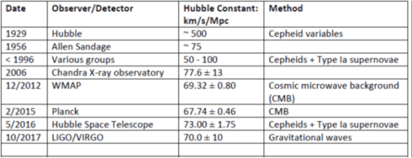
Table 3.2 shows four different methods that have been used to extract H0. The first technique, which we will call the “direct” method, used Cepheid variables; this was utilized by Hubble in 1929 and Sandage in 1956. Between that period and the end of the 20th century, the Hubble constant was extracted mainly using Cepheid variables, supplemented with information from Type Ia supernovae. The latter decades of the 20th century saw a rather contentious debate between a group led by de Vaucouleurs and one led by Sandage. While de Vaucouleurs and collaborators obtained a value near 100, Sandage’s group maintained that the value was more like 50. Each group claimed that the value determined by the competing group was well outside the error bars for these measurements. However, as is apparent from Table 3.2, more recent determinations all obtain a Hubble constant consistent with H0 ≈ 70 km/s/Mpc, with very small error bars, now approaching the 1% level.
More recent techniques for extracting the Hubble constant involve the cosmic microwave background (CMB) radiation and gravitational waves. We will review the CMB in Sections 3.5 and 3.6. At the moment, we can obtain precise values for the Hubble constant from both the Cepheid/supernova data and from the CMB measurements. The gravitational-wave measurements are quite recent, hence these measurements can currently determine H0 to a precision of roughly 10%. From Table 3.2 we see that all the most recent precision measurements obtain a value of H0 between 67 and 73 km/s/Mpc. These values of the Hubble constant imply that all intergalactic distances are increasing at a relative rate of one part per 14 billion each year.
3.4 A Brief Review of the Big Bang Scenario
In this section we review some qualitative features of the Big Bang theory. We reiterate that our explanations are presented here in terms of classical physics arguments; however, all of these features are calculated using Einstein’s General Theory of Relativity.
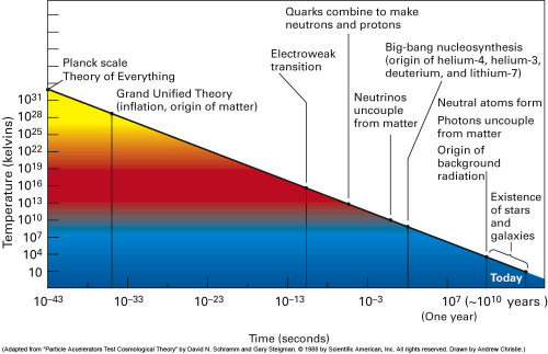
At some instant of time, designated as t=0, the exceptionally hot and dense Universe began to expand. Since that time, the Universe has continued to expand; as it expands, it becomes progressively less dense and cooler. Figure 1.1 (in part I of this series) shows a schematic timeline for the evolution of the Universe in the Big Bang cosmology. Figure 3.4 gives an overview of the average temperature (in Kelvin or absolute temperature) in the Universe as a function of the number of seconds since the beginning of the Big Bang. Note that both time and temperature scales are logarithmic, and that most of the events in Fig. 3.4 take place in less than 1 second after the Big Bang. A number of the milestones that are noted in both Figs. 1.1 and 3.4 are based on the well-established and well-tested theories of the fundamental forces of nature, describing the electromagnetic, strong and weak nuclear interactions.
Very shortly following the Big Bang, the Universe was an exceptionally hot ‘soup’ consisting of particles and radiation. Particles and their corresponding antiparticles were constantly annihilating to form radiation (photons), and vice versa. These reactions are given by the equations
M+M→ γ+γ (3.2a)
γ+γ → M+M (3.2b)
Equation (3.2a) denotes a particle M annihilating with its antiparticle (denoted by M) to produce two photons. Eq. (3.2b) is the inverse of the first reaction, corresponding to production of a particle-antiparticle pair from radiation. A number of different particles with widely varying masses obey similar equations.
These reactions are asymmetric. Using Einstein’s relation between mass and energy, the kinematics of Eq. (3.2a) in the center-of-mass frame are
Mc2 + KEM → Eγ (3.3)
In Eq. (3.3), M is the mass of the particle, KEM is its kinetic energy (assumed here to be equal for particle and antiparticle) and Eγ is the energy of one of the resulting photons. Kinematics for Eq. (3.2b) are the reverse of Eq. (3.2a). Note that particle-antiparticle annihilation reactions (3.2a) can occur for any value of the kinetic energy, even zero. However, production of a particle-antiparticle pair from radiation (3.2b) can only occur when the energy of each photon is greater than Mc2.
Thus, as the Universe expands and the average temperature T decreases as shown in Fig. 3.4, production of heavy particles (large values of M) from radiation will eventually “turn off,” as the average photon energy drops below Mc2.
Matter in the form we now observe in laboratories on Earth would have begun to form during the first few minutes following the Big Bang. The fundamental theories of particle physics tell us that it would have taken only about one trillionth of a second for the Universe to reach temperatures, denoted in Fig. 3.4 as the “electroweak transition,” at which the basic building blocks of matter – the quarks and electrons – first acquired non-zero masses. By this time, it is generally assumed that there was already a very slight (roughly one part per billion) excess of quarks over antiquarks, although the mechanism for this asymmetry is not yet understood. If the numbers of quarks and antiquarks had been identical at this point, the quarks and antiquarks would soon have annihilated each other in pairs. The resulting Universe would end up containing only radiation, and no nuclei or atoms could have been subsequently formed.
About a millionth of a second after the Big Bang the Universe would have cooled to a point where features of the strong interaction changed, so that it became favorable for the remaining quarks (the slight excess that survived quark-antiquark annihilation in pairs) to coalesce to form neutrons and protons. This transition is well understood within the theory known as quantum chromodynamics, and has furthermore been observed in microcosm in the laboratory by colliding heavy nuclei at nearly light speed, at the Relativistic Heavy Ion Collider at Brookhaven National Laboratory on Long Island and at the Large Hadron Collider in Geneva, Switzerland.
When neutrons and protons began to form, the temperature T had already decreased so much that the ambient photons no longer had sufficient energy to produce neutron-antineutron or proton-antiproton pairs (protons and neutrons have nearly identical masses). But since the neutrons and protons had been formed from the very slight earlier excess of quarks over antiquarks, it turns out that there were about a billion photons present for every neutron or proton in the Universe. We infer the value of this ratio from Big Bang explanations of a variety of observations, as we explain below.
A free neutron is unstable; it decays to a proton, electron and electron antineutrino via the process
n → p + e¯ + νe. (3.4)
The half-life of a free neutron is roughly 10 minutes. So, at this point in the evolution of the Universe, neutrons could either decay to protons via the decay process of Eq. (3.4), or they could combine with protons and other neutrons to form nuclei. Inside stable nuclei, the neutrons are bound sufficiently tightly to prevent their radioactive decay. The first step in such building of nuclei would have been the combination of a single proton and a single neutron to form the nucleus of deuterium (a heavier isotope of hydrogen). However, the neutron and proton in deuterium are bound together relatively weakly, and until a time roughly one second after the Big Bang, the ambient radiation still had sufficient thermal energy for a photon to break apart the deuterium nucleus and abort the formation of heavier nuclei.
The era labeled “Nucleosynthesis” in Fig. 1.1 and “Big Bang nucleosynthesis” in Fig. 3.4 thus began about a second after the Big Bang. It ended about three minutes after the Big Bang, because by then the temperature was low enough that different nuclei, each positively charged, no longer had sufficient kinetic energy to overcome their mutual electric repulsion and approach closely enough to fuse. The ambient electrons were able to attach themselves stably to the nuclei formed, to produce electrically neutral atoms, only several hundred thousand years after the Big Bang, because that’s how long it took for the Universe to reach a low enough temperature that photons no longer had sufficient energy to break atoms apart.
From the Big Bang theory, we know the temperature in the Universe at the time nucleosynthesis began. Furthermore, we can determine the rates for protons and neutrons to form atomic nuclei, from experiments performed at particle accelerators. What we don’t know a priori is the ratio at that time of protons and neutrons to photons, that is, of matter to radiation, because that depends on the precise value of the very slight asymmetry between quarks and antiquarks in the infant Universe. Treating that one ratio as an adjustable parameter, one can then calculate the relative abundances of the light nuclei that would have been formed in Big Bang nucleosynthesis. In Fig. 3.5 we show the results of simulations of these relative abundances of light elements as a function of time (upper axis) or temperature (lower axis) of the Universe following the Big Bang. Again, both axes are logarithmic.

Figure 3.5 shows the abundance of neutrons decaying over time. It is evident that the dominant species following the nucleosynthesis process are protons and helium (He4). In fact, calculations in the Big Bang scenario give relative abundances of helium that are very close to 25% of the hydrogen (proton) abundances, as a fraction of total mass. The next most abundant species, deuterium (H2), is roughly 4 orders of magnitude less prevalent than hydrogen. The deuterium production rises rapidly in the early stages of nucleosynthesis, but then falls off in the later stages as deuterium nuclei fuse with other nuclei to form still heavier nuclei. The production of nuclei heavier than helium-4 is severely limited by the detailed energetics of those nuclei and the very short (~3-minute) time window available for Big Bang nucleosynthesis (heavier nuclei are formed in fusion reaction chains within stars, over many thousands of years).
The result in Fig. 3.5 is in striking agreement with experiment. Everywhere we look in the Universe (except inside the cores of stars), we find that hydrogen and helium are the dominant elements, with helium very close to 25% of hydrogen. The agreement between calculations and observations is best when it is assumed that there was one proton or neutron for every 1.6 billion photons present at the start of the nucleosynthesis period. As we will see, that value is in excellent agreement with the value determined completely independently from analyses of the CMB.
The relative abundances of elements are one major reason for the acceptance of the Big Bang Scenario. The Big Bang theory naturally predicts the dominance of hydrogen and helium, and that the helium abundance should be 25% that of hydrogen. It is not possible to extract these abundances accurately and reliably from any competing cosmological scenario, particularly the steady-state theory.
3.5 The Cosmic Microwave Background Radiation
https://en.wikipedia.org/wiki/Cosmic_microwave_background https://map.gsfc.nasa.gov/Universe/bb_tests_cmb.html
https://www.space.com/20330-cosmic-microwave-background-explained-infographic.html
In 1964, physicists Arno Penzias and Robert Wilson were doing research on microwave receivers for use in radio astronomy or satellite communications. They were testing the Holmdel horn antenna microwave receiver, shown in Fig. 3.6. In order to use this receiver for radio astronomy, Penzias and Wilson needed to calibrate the device. It was particularly important to identify and remove background microwave signals from extraneous sources.

Penzias and Wilson found that their receiver was measuring microwave radiation that one would expect to be emitted by a body at a temperature of roughly 2 Kelvin, that is, 2 degrees above absolute zero. The radiation did not seem to be coming from any particular direction in space, in fact it appeared to be uniform from all directions. They attempted without success to determine a source for their “background” radiation, including removing pigeon droppings (along with the pigeons) from their antenna.
Eventually, Penzias and Wilson were directed to Prof. Robert Dicke in the Princeton University physics department. When he saw their results, Dicke immediately realized that Penzias and Wilson had detected “cosmic microwave background radiation” or CMB. At the time, Dicke and his collaborators were in the process of building a radiometer to search for CMB signals themselves. After talking with Penzias and Wilson, DIcke called his collaborators and said, “Boys, we’ve been scooped.” Dicke was correct: in 1978 Penzias and Wilson shared the Nobel Prize in physics for their discovery.
The CMB arises in the following Big Bang scenario, and had in fact been predicted to occur by Ralph Alpher and Robert Herman in 1948. In the early Universe, all atoms are ionized because the ambient radiation has sufficient energy to detach electrons from atoms. However, approximately 400,000 years after the Big Bang the Universe had cooled to the point where radiation was no longer sufficiently energetic to knock electrons from hydrogen. At this point electrons combined with the available nuclei to form electrically neutral atoms. This is the era labeled “Recombination” in Fig. 1.1, and “Origin of background radiation” in Fig. 3.4. At this time the average radiation temperature in the Universe would have been ~3,000 K.
As the Universe continued to expand and cool, radiation in the Universe scattered from neutral atoms (less and less frequently as the expansion proceeded) rather than ionizing them. Before this time, the Universe was opaque to visible light (there was a white-hot fog of glowing hydrogen plasma); afterwards, the Universe became transparent to visible light. The subsequent process of scattering produced a thermal or black-body spectrum of radiation corresponding to T ~ 3,000 K. In the intervening epochs since this time, up until today, all cosmic distances have expanded by a factor of 1,100. The wavelength of the photons last scattered around the time of recombination has increased by an identical factor, while their density has decreased by a factor of (1,100)3 as cosmic volumes have increased by that factor. These changes combine to alter the spectrum of energy density contained in radiation within the Universe in precisely the same way as would the cooling of a black-body by a factor of 1,100, from an initial temperature of 3,000K to about 2.7K.
The CMB spectrum has now been measured with spectacular precision. It is shown in Fig. 3.7. The curve is a black-body spectrum calculated for a mean temperature T = 2.725K; these temperatures correspond to wavelengths currently in the microwave sector of the radiation spectrum, hence the name “cosmic microwave background radiation.” The data points are from the COsmic Background Explorer (COBE) satellite. Up to the 1990’s, this was the most precise black-body spectrum ever observed. Most of the radiation energy in the Universe is currently found in the CMB.
The existence of cosmic background radiation was predicted in 1948 by Alpher and Herman. They initially estimated the present temperature of the CMB spectrum at about 5 K; however, in a later paper they revised this to 28 K. We now understand that Alpher and Herman’s large value was due to their use of an incorrect value for the Hubble constant.
The CMB prediction of Alpher and Herman was then forgotten for several years before it was re-discovered by Zel’dovich in the early 1960s, and also by Dicke at about the same time. Measurement of the CMB and its black-body spectrum represented spectacular confirmation of the Big Bang scenario. No competing cosmological theory predicted the existence of such a spectrum. The continuous expansion of cosmic space that is embedded in the Big Bang theory is essential to maintain a precise black-body spectral form, even as the temperature cools by orders of magnitude. Furthermore, the mean temperature of the CMB spectrum measured today is in excellent agreement with our current understanding of the origin and history of the Universe.

3.6 Fluctuations in the CMB Spectrum
Following the discovery of the CMB radiation it was realized that, despite the precision of the black-body temperature spectrum, the radiation arriving at Earth from different directions in space should show tiny fluctuations in temperature. The argument goes as follows. In early times following the Big Bang, mass was distributed nearly uniformly throughout the Universe. However, there existed regions of space with slightly greater mass density than the mean, and regions with lower mass density. Through the self-organizing property of gravity, regions with slightly larger mass density will attract more and more matter from surrounding regions. Eventually, the high-density regions will accrete sufficient mass to form galaxies.
Prior to the recombination era, when ambient photons would have been interacting continually with electrically charged nuclei and electrons, these interactions would have been slightly more frequent in the regions of higher mass density. Those more frequent interactions would have led to slight relative heating of the more dense matter. At the same time, the competition between the outward pressure from those interactions and the attractive force of gravity would have led to pressure waves (otherwise known as sound waves) propagating outward like ripples from pebbles dropped in a pond. Those sound waves would have carried some of the matter from the overdense regions outward, until the recombination epoch when the frequent photon interactions and the outward pressure ceased. The early Universe sound waves are called “baryon acoustic oscillations” (BAO). Those density fluctuations and sound waves in the early Universe would have provided the matter seeds for the large-scale structure (galaxies, galaxy clusters and superclusters) we observe in today’s Universe.
One can carry out simulations of mass distributions in the early Universe. We know the current density of galaxies in the Universe, and the distribution of galactic masses. From this, we can work backwards to determine the size of mass density fluctuations in the early Universe that would lead, over billions of years of gravitational attraction, to the current distribution. When these simulations are carried out, it turns out that early mass density fluctuations of a few parts in 100,000 would produce a current Universe similar to our own.
So, experiments were launched to make precision measurements of fluctuations in the CMB black-body temperature spectrum. One such experiment was the COBE satellite that operated from 1989 to 1993. It was designed to measure fluctuations in the CMB spectrum. Fig. 3.8 shows a map of the sky with COBE temperature results. Red areas have higher mean temperatures than average, while blue areas have lower T. The observed temperature fluctuations shown in Fig. 3.8 are in parts per 100,000, in good agreement with simulations of mass distributions in the early Universe. Two of the principal investigators of COBE, George Smoot and John Mather, were awarded the 2006 Nobel Prize for their work: the Nobel Prize citation credited their project as “the starting point for cosmology as a precision science.”

Two even more advanced spacecraft followed on to the COBE measurements: these were the Wilkinson Microwave Anisotropy Probe (WMAP) detector that operated from 2001 – 2010, and the Planck detector from 2009 – 2013. These projects have made the delineation of fluctuations in Fig. 3.8 much more precise. These in turn were supplemented by two balloon telescope measurements of CMB anisotropies — the BOOMERanG telescope (1997 – 2003) and the Maxima experiment (1998 – 1999).
3.7 The Big Bang Scenario and Fits to Cosmological Data
Today, one has a wealth of precision data from dedicated cosmic background experiments such as COBE, WMAP, Planck and the balloon measurements. These radiation data can be combined with ever more precise observational data from both ground-based telescopes and space detectors such as the Hubble Space Telescope, that produce detailed maps of the distribution of matter in the Universe. This combination of radiation and matter measurements now provides an extraordinary amount of information on the history of the Universe, to test the Big Bang scenario.
Information (electromagnetic radiation and, most recently, gravitational waves) from distant objects travels at the speed of light to Earth. The farther this information has traveled, the earlier the events whose information is now reaching us. The recession velocity of a distant galaxy is characterized by a redshift value z, which specifies the fractional increase in the wavelength of light from the time of emission to the time of detection on Earth. The quantity z+1 then tells us the factor by which cosmic distances have increased since the emission of the light, and in Big Bang cosmology this is equal to the factor by which the temperature of the Universe has decreased since the emission of the light. This allows us to check our hypotheses regarding the origin and history of the Universe, expressed in the timeline of Fig. 1.1. As we pointed out in Sect. 3.4, the abundances of light elements allow us to check the “Nucleosynthesis” era. The existence and properties of the CMB validate the “Recombination” era, corresponding to z ≈ 1100. In addition, we are now able to directly observe signals out to z ≈ 6 from the earliest visible galaxies that formed roughly 700 million years after the Big Bang, when cosmic distances were about one-seventh their present size.
Recent observations have allowed us to fill in previously missing details of the Big Bang scenario. First, we can now make very precise measurements of the mass-energy density in the Universe. This has led to two major surprises. The first is the existence of “dark matter”. This is a form of matter different from “normal” matter, comprised of protons, neutrons, electrons, neutrinos and nuclei. Dark matter does not interact with electromagnetic radiation, so we cannot see it directly. But it does exert gravitational forces, just like ordinary matter, and we can detect its presence by virtue of these forces.
The existence of dark matter was first inferred, from the 1930s onward, from the systematics of persistently high orbital speeds observed for stars in outer reaches of many galaxies. The distribution of dark matter within the Universe has more recently been determined indirectly from “gravitational lensing” experiments. In his General Theory of Relativity, Einstein showed that the path of light and EM radiation is bent by the presence of matter. As light from a distant object passes large masses on its way to us, that light is bent as if by a lens, forming identifiable images. Observation of the bending of light from distant visible sources can thus be used to determine the spatial distribution of mass along the light’s path, whether or not that intervening mass is itself visible.
A second recent surprise is that the expansion of the Universe is currently accelerating. This was first observed in 1998 through measurements of the motion of distant Type Ia supernovae by groups led by Perlmutter, Schmidt and Riess, who shared the 2011 Nobel Prize for this discovery. That observation has since been confirmed by both gravitational lensing experiments and by precision measurements of the CMB by the WMAP and Planck satellites and by BOOMERanG and Maxima balloon telescopes. Their results, plus more recent measurements from a number of detectors, for the “power spectrum” (the amplitude of temperature differences between two directions as a function of their angular separation) of the CMB are shown in Fig. 3.9.

The power spectrum of Fig. 3.9 shows several clear peaks in the angular scale of CMB temperature fluctuations. The detailed structure of that power spectrum contains a wealth of information about the distribution of matter and energy in the early Universe, including the distance covered by the outgoing BAO sound waves by the time recombination occurred, about the expansion history and age of the Universe, and about the geometry of space. The total energy density of the Universe, including energy in all forms, determines the geometry of space, i.e., whether space is convex, concave or flat.
According to General Relativity, cosmic space can be flat only if the total energy density in the Universe maintains a critical relationship to the Hubble constant as cosmic distances expand and both values evolve with cosmological time. From current measurements such as those in Fig. 3.9, we can deduce that the total energy density of the Universe is equal to this critical density within a current experimental uncertainty of about 0.5%. So space appears to be flat as far out as we can see, to a horizon limited by communication at the speed of light within the finite age of the Universe. (The Universe may extend well beyond this horizon, but we cannot currently obtain information from beyond it.)
However, the so-called 2dF Galaxy Redshift survey in 2001 found that the matter density for normal and dark matter combined is roughly 30% of the critical density. The disagreement between the CMB fluctuations and the Galaxy Redshift results suggested that there might be an additional contribution to the energy density in the Universe, over and above the known contributions from matter and radiation. Furthermore, the accelerated expansion results from Perlmutter et al. indicated the existence of some force of unknown origin that was causing objects in the Universe to repel each other to produce the accelerated expansion, in competition with the attractive force of gravity. The force leading to that repulsion would contribute to the energy density in the Universe, a contribution labeled as “dark energy” to emphasize our lack of clear understanding of its source.
The simplest account for this repulsive force is via a cosmological constant. This was a concept introduced by Einstein into his General Theory of Relativity in 1917. At the time, Einstein postulated a static Universe where the galaxies were at rest. However, such a Universe would collapse because of the mutual gravitational attraction of all the matter within it. So Einstein introduced an ad hoc cosmological constant – an energy density that did not change over cosmological time – that provided effective repulsive forces to prevent the Universe from collapsing. However, once Einstein became aware of Hubble’s results that showed an expanding Universe, he dropped the cosmological constant as it now appeared extraneous, and reportedly referred to its earlier inclusion as his “biggest blunder.” However, the presence of a cosmological constant could account for the current accelerating expansion of the Universe. In an expanding Universe, the cosmological constant represents a continual source of dark energy, since it must maintain a constant energy density even as cosmic volumes grow.
Astrophysicists have now developed a “standard model” of cosmology to describe the origin and evolution of the Universe. This is called the Lambda-CDM (Lambda-cold dark matter) model. The “Lambda” refers to the cosmological constant. The cold (slow-moving, presumably because it is composed of quite massive particles) dark matter provides the initial seeds that gravitationally attract faster-moving ordinary matter to begin the formation of stars and galaxies. This model is capable, with a small number of adjustable parameters, of accurately explaining a large number of observed astrophysical phenomena. It can explain the existence and structure of the cosmic microwave background; the large-scale structure in the distribution of galaxies, arising from the initial tiny density fluctuations in the infant Universe; the abundances of light elements (seen in Fig. 3.5); and the accelerating expansion of the Universe observed in the light from distant galaxies and supernovae.
The Lambda-CDM model contains a number of parameters that are varied to provide the best fits to cosmological data. In concert with the Standard Model of particle physics, this cosmological model can describe most of the epochs shown in Fig. 1.1, starting from a time of about 10-32 seconds following the Big Bang. (Understanding the Universe’s evolution at even earlier times requires advances in both particle physics theories and a treatment of the “beginning” of the Big Bang, such as the concept of “cosmic inflation” to be described later in this blog post.) In many ways, the Lambda-CDM model is spectacularly successful. For example, in Fig. 3.9 the data points are a compilation of all measurements of the CMB anisotropies, while the solid curve is the best Lambda-CDM calculation, obtained by varying 6 basic parameters. You can try adjusting these parameters yourself to see how they affect the power spectrum at https://map.gsfc.nasa.gov/resources/camb_tool/cmb_plot.swf.
The Lambda-CDM model provides tight constraints on the mass and total energy density in the Universe. Currently, the best values imply that 4.9% of mass-energy density arises today from normal matter, that is, from atoms; 26.8% comes from cold dark matter; and 68.8% comes from dark energy. Approximately 0.01% of the energy density today comes from CMB radiation, and no more than 0.5% arises from relic neutrinos. However, these fractions would have varied dramatically during the history of the Universe, because the matter density and radiation energy density have different dependences on the cosmic distance scale, while the dark energy density is unchanging in the Lambda-CDM model. Thus, the infant Universe would have been radiation-dominated, but the matter energy density would have overtaken it some 50,000 years after the Big Bang. The dark energy density became comparable to the matter energy density some 6 or 7 billion years ago, at which point the expansion of cosmic space changed from deceleration to acceleration.
One of the variables in the Lambda-CDM model is the current value of the Hubble constant. We refer to values for the Hubble constant extracted from these fits as “indirect measurements” of the Hubble constant. For example, in Table 3.2 the WMAP and Planck extractions of the Hubble constant arise from these cosmological model fits. The Hubble constant can now be extracted with increasingly greater precision. In Fig. 3.10 we show the most recent values obtained for H0. The blue points represent Hubble constant values from “direct” measurements (recession velocities of Cepheid variables, Type 1a supernovae, plus the tip of the red-giant branch – this is another technique in the ‘cosmic distance ladder’). These measurements appear to be converging to a Hubble Constant of roughly H0 = 73 km/sec/MPc with a precision of approximately 3%.
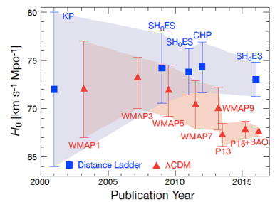
On the other hand, Hubble constant values extracted from cosmological fits using the Lambda-CDM model now obtain “indirect” values such as H0 = 69.8, with a statistical uncertainty of about 1.5%. As the precision of each method has improved in recent years, the direct and indirect values for H0 have begun to differ slightly, by about 3 standard deviations. This suggests that either some parameter(s) in the Lambda-CDM model need to be adjusted (for example, that the dark energy density is not constant over cosmological time), or that systematic uncertainties in the direct-measurement analyses are larger than currently assumed.
Regardless of these slight differences in the Hubble constant, the age of the Universe (the time since the Big Bang) is now determined with great precision. That time can be extracted from the cosmological models. The Planck satellite measurements found that the age of the Universe is 13.82 billion years; the WMAP extraction of this number was 13.72 billion years. So cosmological models determine the age of the Universe to about 1% precision.
The same Lambda-CDM model fits to the CMB power spectrum also allow one to determine the ratio of the density of protons and neutrons to that of photons at the time of Big Bang nucleosynthesis. The result is in complete agreement with, but is more precise than, the value extracted by fitting Big Bang nucleosynthesis calculations to observed light-element abundances in today’s Universe. The agreement between these two independent determinations provides another testimonial to the basic correctness of Big Bang cosmology.
The past 25 years have seen an explosion in the amount of precision cosmological data. This has enabled scientists to determine fundamental astrophysical constants to unprecedented precision. To be sure, there are still major unanswered questions in this field. The latest cosmological models are consistent with a period of extraordinarily rapid expansion in the infant Universe, called “inflation” in Figs. 1.1 and 3.4. The concept of cosmic inflation helps to explain how the Universe may have come to be so uniform and so flat, but there is as yet only weak circumstantial evidence for such an inflationary period. Although the overall matter density of dark matter is measured with great precision, the nature and composition of dark matter is also not yet well understood. And the nature of dark energy is even more mysterious. Finally, we do not yet understand the origin and magnitude of the quark-antiquark asymmetry in the early Universe, which has prevented a matter-free Universe. Many experimental searches and theoretical speculations are currently under way to gain further insight to these features of cosmology. However, the age of the Universe does not depend on the depth of our understanding of these concepts. The age of the Universe depends on a number of extremely well-measured quantities and it is currently determined to within 1% precision.
