The Ozone Layer Controversy, Part I

Update Apr. 2023: New developments on ozone-depleting chemicals in the atmosphere. A paper in Nature Geoscience 2023 by Luke Western et al. points out that between 2010 and 2020, five chlorofluorocarbons (CFCs) have been increasing in the atmosphere, despite the worldwide ban on CFCs required under the Montreal Protocol. These five chemicals are CFC-13 (CClF3), CFC-112a (CClF2CCl3), CFC-13a (CF3CCl3), CFC-114a (CF3CCl2F) and CFC-15 (CF3CClF2). Of these five chemicals, three of them (CFC-13a, CFC-14a, and CFC-15) are known “feedstocks,” or intermediate states or by-products during the production of other chemicals. The most notable target chemicals that might include these CFCs as intermediate states are the two most common hydrofluorocarbons (HFCs), HFC-134a and HFC-125. The origin of two of the CFCs, CFC-13 and CFC-112a, is uncertain.  The authors speculate that the increase in CFC-13 may be because it is a by-product during the production of CFC-11. The source of the chemical CFC-112a is unknown; the authors hypothesize that it may be a feedstock for fluorovinyl ether production.

Previous research has identified East Asia as the source of CFC-113a and CFC-15 emissions. At present, the impact of these chemicals on stratospheric ozone is modest. Cumulative emissions of these five chemicals relative to 2010 levels could result in a loss in global stratospheric ozone of approximately 0.002%, or a loss of 0.01% in ozone in the Antarctic Spring.  However, if emissions of these five CFCs continue to rise, they may negate some of the benefits that have been gained under the Montreal Protocol.

Update Jan. 2023: New developments on the ozone layer.

Under the terms of the Montreal Protocol, every four years an international Scientific Assessment Committee releases a report summarizing the current state of the ozone layer and efforts to monitor the effects of chemicals that have the potential to destroy the ozone layer.  The latest 2022 report was issued in Jan. 2023, and contains some very encouraging findings.

The Montreal Protocol established means by which production of CFCs would be banned, and in addition offered both scientific support and financial incentives from developed countries to Third-World countries to assist them in transitioning from production of CFCs. Following actions taken by all nations on Earth, the hole in the ozone layer which is described in this post is on track to be completely healed within about two decades.  The report states that by 2040, the ozone layer at mid-latitudes should be completely recovered to its status before the release of chlorofluorocarbon chemicals (CFCs).  The ozone layer over the poles will recover somewhat more slowly (for reasons described in this post); in the Arctic region, the ozone layer should fully recover by 2045, and the Antarctic ozone layer should be fully healed by 2066.

After most countries began to halt the production of chlorofluorocarbon chemicals in the early 1990s, the initial findings suggested that the ozone hole would slowly but surely heal over the next 60 years.  However, in 2018 scientists discovered that CFC releases had continued.  This was traced to sources in China, and eventually these chemicals were banned.  As described in our post the chemicals that replaced CFCs, hydrofluorocarbons or HFCs, were highly successful in maintaining the ozone layer.  Unfortunately, many HFCs turned out to be very strong greenhouse gases.  In 2019, governments agreed to replace HFCs by chemicals that were much less harmful as greenhouse gases, through the Kigali Amendment to the Montreal Protocol.

Petteri Taalas, the secretary-general of the World Meteorological Organization, stated that “Our success in phasing out ozone-eating chemicals shows what can and must be done as a matter of urgency to transition away from fossil fuels, reduce greenhouse gases and so limit temperature increase.”  David Fahey, a lead author of the 2022 Scientific Assessment, stated that the Montreal Protocol is “The most successful environmental treaty in history and offers encouragement that countries of the world can come together and decide an outcome and act on it.”

July 19, 2017

Review of the Ozone Layer Controversy

At this moment, controversy over global climate change is likely the most contentious scientific issue faced by American society. Currently, positions between the two sides have hardened, and differences of opinion have now become fractured along political party lines. Both sides now claim to have responsible scientific evidence on their side. In order to determine which side is accurately representing the evidence, it will be instructive to review an earlier controversy: potential human-caused threats to the ozone layer.  This is the issue that we will review in this blog post. As we shall see, many of the issues that arise in the climate change debate are also evident in the ozone layer controversy.

An advantage of “looking back” at the ozone layer controversy is that its scientific questions are now mainly settled. Furthermore, the results of scientific experiments and improved monitoring allow us to review competing theories of effects on the ozone layer. And finally, we examine statements by “denialists” who challenge the prevailing scientific hypothesis.

We will see that some groups and individuals who fought against the consensus of the scientific community on the ozone layer are the same people who are active in denial of global climate change. And indeed, many of the arguments against the scientific consensus on ozone are identical to those raised in the current debate over climate change.

In preparing this summary, we made extensive use of the summary of the Ozone Depletion story from the Berkeley series at www.understandingscience.org We quote from the summary of the ozone controversy by William Brune. We also used the monograph Merchants of Doubt, by Oreskes and Conway. We reference comments by S. Fred Singer from his 2010 Heartland Institute publication. And finally we use material from the blog post The Skeptics vs. The Ozone Hole, by Jeffrey Masters. All of these are referenced in the list of Source Materials at the end of this blog post.

1.  CFCs and the Atmosphere

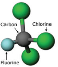
Chlorofluorocarbons (CFCs) are organic compounds that are made up of chlorine, fluorine and carbon in varying amounts. A schematic picture of a CFC molecule is shown in Fig. 1.

CFCs were developed in the late 1920s in an effort to produce non-toxic substances that could be used as refrigerants. The boiling points of CFCs made them useful for refrigerants. The most widely-used refrigerant was the product Freon, manufactured by the DuPont chemical company. Freon was used as the coolant in air conditioners, and in refrigerators.

In addition, CDCs were widely used in aerosols; they formed the propellant in spray cans. They also appeared in foam insulation. Products such as polystyrene cups and “packing peanuts” were manufactured in processes that used CFCs. And CFCs were also used as cleansers for electronic components. As of the 1970s, up to 10 billion pounds per year of CFCs were being manufactured.

Until 1970, it was not known whether CFCs were entering the atmosphere. British scientist James Lovelock developed an instrument capable of detecting trace amounts of CFCs in the atmosphere. Lovelock initially found CFCs in urban areas; however, later tests found CFCs over the Atlantic Ocean. This demonstrated that CFCs were being carried around the world by large-scale air currents.

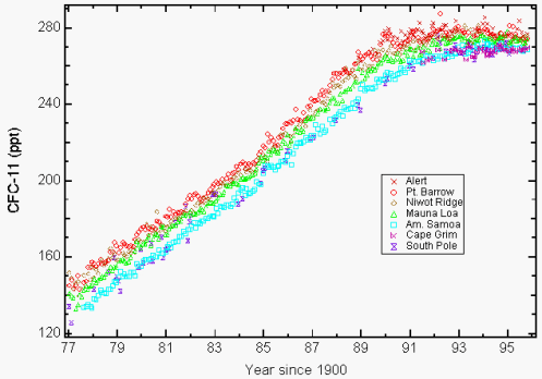
Fig. 2 shows measurements of atmospheric concentrations of a particular molecule, CFC-11, vs. time. Measurements were taken at seven different locations around the globe; all show extremely similar behavior. Also, the measured CFC concentrations closely track the changing annual usage of CFCs, with some time lag because of the persistence of CFCs in the atmosphere.

Atmospheric chemist F. Sherwood (“Sherry”) Rowland of the University of California, Irvine, was curious when he heard about Lovelock’s measurements. He knew that CFCs were particularly stable, and together with colleague Mario Molina decided to investigate what would happen to CFCs once they entered the atmosphere.

Rowland and Molina discovered that in the lower atmosphere, CFCs could remain for decades. The chemicals were nearly insoluble in water, resistant to oxidation, and unaffected by sunlight in visible wavelengths. Through mixing in the atmosphere, CFCs would gradually rise into the stratosphere. There, the CFCs would rise until they reached the level of the ozone layer.

2.  The Ozone Layer

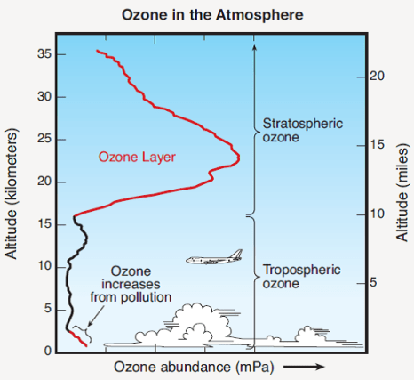
At an altitude of 10-50 kilometers above the Earth (this number depends on the latitude), concentrations of ozone (the molecule O3) increase dramatically. Concentrations of ozone vs. altitude are shown in Fig. 3.

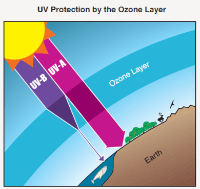
The region with the highest concentration of ozone is called the “ozone layer.” The process leading to formation of ozone is shown in Fig. 4. Ultraviolet (UV) radiation from the Sun, especially the short-wavelength UV-B rays in the wavelength range 280 – 315 nanometers (nm), interacts with a molecule of oxygen O2. The UV-B ray is absorbed, and its energy is transferred to the oxygen molecule, which splits into two oxygen atoms.

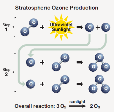
Each of the oxygen atoms subsequently combines with an oxygen molecule to form a molecule of ozone. In the overall process, three oxygen molecules react with UV-B sunlight to form two molecules of ozone.

At this level in the atmosphere, the production of ozone by UV rays, and the destruction of ozone by other chemical reactions, results in equilibrium levels of ozone, oxygen molecules and oxygen atoms. Note that at these altitudes, the oxygen molecules are very effective absorbers of UV-B rays.

Thus, above the ozone layer, sunlight contains relatively high concentrations of UV-B rays. However, below the ozone layer, levels of UV-B decrease dramatically. This is shown in Fig. 5. As a result of the ozone layer, very few UV-B rays reach the surface of the Earth. The presence of the ozone layer thus has significant health benefits for the Earth.

UV-B rays produce skin cancers, cataracts and suppressed immune systems in humans and animals; they also have deleterious effects on terrestrial plants and aquatic ecosystems.  This is apparent from Fig. 6, which shows the effects of different wavelength light in producing skin damage.

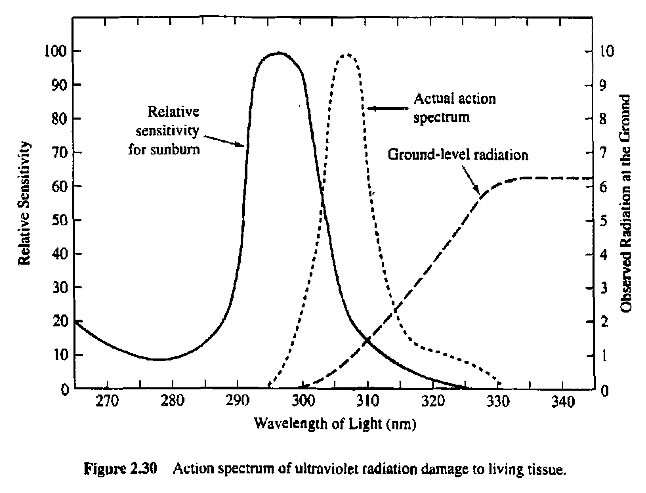
In Fig. 6, the solid curve shows the ability of light to produce sunburn as a function of its wavelength. The long-dashed curve shows the intensity of observed radiation that reaches Earth’s surface. The actual effects of various wavelengths of UV light to damage living tissue (the short-dashed curve in Fig. 6) are obtained by weighting the sensitivity curve (solid) by the intensity of ground-level radiation (long-dashed). It is clear that the skin damage from sunlight at ground level is highly concentrated in the UV-B (280-315 nm) region.

Thus the presence and thickness of the ozone layer protects us from the hazards of UV-B rays. Note that the ozone layer has a far less dramatic effect on the longer wavelength (315 – 400 nm) UV-A rays, but these are relatively ineffective in damaging living tissue.

3.  CFCs and the Ozone Layer

Rowland and Molina predicted that once CFCs reach a sufficiently high altitude, at or above the ozone layer, the dramatically increased levels of UV-B radiation would be sufficient to break down a CFC molecule, releasing an atom of chlorine. That process is shown schematically in Fig. 7.

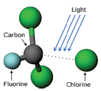
Although CFC molecules are essentially unaffected by sunlight in the visible wavelengths, the photons associated with UV-B rays have sufficient energy to allow the process in Fig. 7 to proceed.  (Photon energy increases as the wavelength decreases.) Thus, once CFCs reach the level of the ozone layer or above, the strong intensity of UV-B rays could cause CFCs to break down and release free chlorine atoms.

Once a free chlorine atom is released, it can interact with ozone as shown in the cartoon of Fig. 8. In the top row, an atom of chlorine interacts with an ozone molecule, producing a molecule of oxygen plus chlorine monoxide (Cl O).

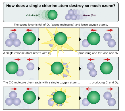
The Cl O molecule then interacts with an oxygen atom; the result of this reaction is a molecule of oxygen plus a chlorine atom (2nd row of Fig. 8). That chlorine atom is then free to interact with and destroy another ozone molecule.

A single chlorine atom freed from a CFC has the potential to destroy up to 100,000 ozone molecules. At the time they considered this possibility, Rowland and Molina were unaware that the chlorine atom chain reaction on ozone had recently been observed experimentally by Stolarski and Cicerone.

In 1974, Rowland and Molina published a paper suggesting that the continued release of CFCs into the atmosphere would be likely to decrease levels of stratospheric ozone by 7 to 13 percent by the year 2050. Health officials estimated that every 1 percent reduction in the ozone layer might produce a 6 percent increase in skin cancers and cataracts. If the predictions by Rowland and Molina were correct, then it would be dangerous to continue releasing CFCs into the atmosphere.

4.  Research and Monitoring by the Scientific Community

Spurred on by the hypothesis from Rowland and Molina, the scientific community mounted a coordinated world-wide effort to monitor CFCs and ozone in the atmosphere. In particular, it would be essential to determine whether CFCs were reaching the ozone layer, if they were breaking down at that altitude due to interactions with UV light, and whether the ozone layer was adversely affected by CFCs.

In addition, one would need to assess how long CFCs would remain in the atmosphere. Would they persist for up to 100 years as suggested by Rowland and Molina, or might there be some hitherto-unknown mechanism capable of breaking down CFCs before they reached the ozone layer?

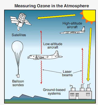
Fig. 9 shows various methods for measuring ozone in the atmosphere. Depending on the altitude, a number of different methods are available to measure ozone concentrations. It is particularly important that different measurements performed at the same altitude should agree with one another.

It took only a short period of time to verify in the laboratory the hypothesis that UV light could break down CFCs and release chlorine atoms. Such experiments were carried out at the National Bureau of Standards.

In 1975, measurements from both balloon-borne instruments and high-altitude aircraft measured CFC concentrations at different altitudes in the atmosphere. Both results showed that CFCs reached levels in the upper atmosphere, in agreement with the notion that the CFCs were not being destroyed at lower altitudes by any chemical processes.

However, when the CFCs reached a certain altitude (consistent with the location of the ozone layer), levels of CFCs dropped. These rates were in quantitative agreement with the Rowland-Molina hypothesis that at these altitudes, CFCs were being destroyed by UV light.

It took a longer time to prove that chlorine from CFCs was in fact destroying ozone in the upper atmosphere. A “smoking gun” that this reaction was occurring would be the presence of chlorine monoxide (see the right-hand column, first row of Fig. 8).  But in 1974 it was not possible to test for Cl O at high altitudes.

However, an instrument was soon constructed, and by 1976 James Anderson was able to measure levels of Cl O in the ozone layer. Anderson’s results of the ratio of chlorine to Cl O were close to the value expected if the hypothesis of Rowland and Molina was correct. This strongly suggested that chlorine from CFCs was being liberated by UV light, and destroying ozone via the mechanism shown in Fig. 8.

5.  What About Volcanoes?

An alternative explanation for chlorine in the stratosphere might be emissions from volcanic eruptions. Volcanoes can emit massive amounts of hydrochloric acid (H Cl). How much of the hydrochloric acid released by volcanoes reached the stratosphere, and could it be a major source of the detected chlorine in the ozone layer?

Although volcanic activity can release huge amounts of H Cl, the vast majority of volcanic chlorine is released in the form of volcanic ash, most of which falls back to Earth before reaching the stratosphere. A significant amount of volcanic chlorine is dissolved in water vapor, and again does not reach the stratosphere.

One can compare levels of stratospheric chlorine with major volcanic eruptions. For example, following the eruption of El Chichon in 1982, levels of H Cl in the stratosphere increased by less than 10%. The much larger eruption of Pinatubo in 1991 increased stratospheric chlorine even less. Yet stratospheric H Cl levels increased steadily between these two events, in the absence of any other major volcanic eruptions.

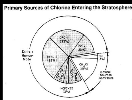
Fig. 10 shows the bottom line concerning sources of measured chlorine levels in the stratosphere. The shaded area is human-made sources, primarily from various CFCs. The unshaded area is from natural sources, including chlorine from volcanoes. The total stratospheric chlorine contribution from natural sources is less than 20%.

6.  The Hole in the Antarctic Ozone Layer

Since 1957, researcher Joseph Farman had collected atmospheric samples in Antarctica. In 1982, he discovered a dramatic dip, nearly 40%, in ozone abundances. Since this decrease appeared inconsistent with satellite data, Farman began checking his results from earlier periods. He discovered that ozone declines had started around 1977. Farman’s annual data from the month of October are shown in Fig. 11.

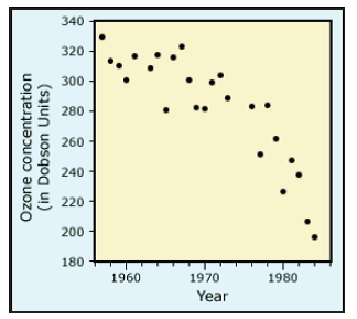
Although there is considerable scatter in the data in Fig. 11, reflecting seasonal and annual fluctuations from other sources, nevertheless there is a noticeable decrease beginning around 1977. After 1977, it is obvious that average October Antarctic ozone levels systematically decrease every year.

Since Farman’s results came from just a single location, his group then took measurements from a second site 1,000 miles away. They obtained the same results. They then compared their results with NASA satellite data that appeared to show no such decrease in ozone levels.

Eventually, it was realized that the NASA satellites had been programmed to filter out measurements with large deviations from “expected” results. The assumption was that such deviations would necessarily result from faulty measuring equipment. When the NASA analysis programs were corrected, their measurements showed a massive hole in the ozone layer above the Antarctic. The NASA measurements now agreed with Farman’s ground-based results.

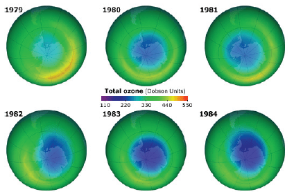
Fig. 12 shows measurements by NASA of the “hole” in the ozone layer over the Antarctic, as a function of time. Because of seasonal fluctuations in the ozone layer, measurements are compared every October. The area of the depleted ozone region is roughly the size of the United States.

The discovery of the hole in the Antarctic ozone layer dramatically changed the debate over ozone depletion. Some hitherto-unpredicted chemical process was causing the ozone layer to be depleted at a much higher rate than was expected. Since the depletion was growing in both magnitude and area covered, this was particularly disturbing to Southern Hemisphere inhabitants such as those in New Zealand and Australia.

Susan Solomon speculated that the ozone layer hole might be caused by the presence of high-altitude clouds of ice particles that exist over Antarctica. She and colleague Rolando Garcia constructed an atmospheric model that included ice particles. Their model predicted that the solid surfaces of ice crystals would greatly increase the destruction of ozone by CFCs.

On the ice surfaces, inert chemicals such as CFCs interacted to form highly reactive chlorine compounds, that would then destroy ozone. Collaborating with Rowland and Molina, Solomon showed that chlorine would destroy ozone at a much faster rate in the presence of ice crystals.

This model predicted that ozone would also be depleted over the Arctic, where ice clouds are also present but in smaller abundance than in the Antarctic. Indeed, ozone “holes” in the Arctic were also detected, and the magnitude of ozone depletion was smaller than in the Antarctic. This supported the notion that the ice clouds were responsible for rapid ozone depletion.

One additional piece of evidence was the understanding of the role played by the polar vortex. The polar vortex is caused by powerful winds that circulate around the pole. The vortex confines the ozone-depleted region to remain over the Antarctic, and impedes the movement of undepleted air from mid-latitudes to the Antarctic.

A final step was to measure levels of both chlorine monoxide and ozone in the ozone layer. James Anderson of NASA mounted a detector on the wing of a plane, and flew the plane through the region of the Antarctic hole. His data are shown in Fig. 13.

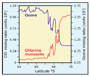
In Fig. 13, the data on the left are obtained outside the Antarctic ozone hole region, while the data on the right are inside the ozone hole. Inside the ozone hole, levels of ozone are low while those of Cl O are high, whereas the opposite is true outside the ozone hole. This further strengthens the link between chlorine and ozone depletion.

Finally, alternative hypotheses were advanced to account for the hole in the Antarctic ozone layer. One of these was that natural variations in UV solar radiation were responsible for the hole. A second was that the hole was caused by changing circulation patterns in the atmosphere. Both of these were tested and found not to explain this phenomenon.

7.  Worldwide Ozone Depletion

The Antarctic ozone hole had been measured by both ground-based and satellite detectors. It was clear that the magnitude of the ozone hole was growing with time, and was apparently caused by chlorine in the stratosphere. This raised a question why ozone depletion had not been observed at mid-latitudes.

Ground-based measurement stations had been tracking ozone levels at various locations around the globe since the 1950s. No reduction in ozone levels had been detected. To understand this apparent discrepancy, in 1987 NASA organized the Ozone Trends Panel, consisting of 150 scientists from around the world.

The Ozone Trends Panel re-evaluated the ground-based data and concluded that there was an average annual ozone depletion of 1.7 – 3% in the Northern Hemisphere. This had not already been observed because previous analyses had assumed that the amount of ozone depletion would be the same throughout the year, and the same at all latitudes. Thus, measurements taken at different times of year and at different latitudes had been lumped together and averaged.

Now that it was understood that ozone depletion might have significant seasonal variation, data from different months and from different latitudes were analyzed separately. From Fig. 11, it is clear that ozone data has considerable “scatter.” In this re-analysis, the small mid-latitude decrease could be observed and quantified.

So, by the early 1980’s ozone depletion had been established and the probable cause from CFC use identified.  How did the international community and the chemical industry react?  That will be treated in Part II of this blog post…