
January 21, 2021
In this part we provide answers to the critical thinking questions posed in Part I. For some of the questions, we provide some talking points that might appear among others in a complete answer to the question posed. Where appropriate, we offer the reasoning to back up the response we provide. Refer back to Part I to see the full questions.
I. Questioning Assumptions
- It is normal to make the implicit assumption that the blind beggar is male. But this assumption is not justified, when you are told that “brother” is not the right answer. In this instance, then, the blind beggar must be female, and therefore the sister to her brother who died.
2) The doctor made two assumptions here. The first is that no woman has two appendices, which is a very good assumption. The second is that the caller is married to the same woman who was his wife eight years earlier, and that assumption is questionable. The husband, on the other hand, is making the good assumption that he knows how to recognize the symptoms of appendicitis, since he has previously experienced them himself and with his former wife. He was well justified in taking his new wife to the emergency room.
3) There is no solid basis for assuming that the trend in 100-meter dash times is linear. Rather, it is quite likely to flatten out at some point, for both men and women. Furthermore, even if you do assume a linear dependence on year, the data do not define the slope of that line very precisely, as indicated clearly by the change from the red to the orange best-fit line when adding data from three additional Olympics. Since the authors are extrapolating a very long way to get to their predicted crossing point, uncertainties in the slope of the lines lead to a very large uncertainty in the year the two lines would cross, if in fact the trends remained linear. One should therefore place little credence in the prediction that women will overtake the times of male runners by 2156.
II. creative problem solving
4) The optimal solution is to connect with all three people waiting for the bus. The driver can do this, for example, by loaning his car keys to his old friend and asking that friend to drive the old woman, as the one passenger the car will accommodate, quickly to the nearest hospital. In the meantime, the original driver can connect with the “perfect partner” as they both wait for the bus that will take them to the hospital, where they meet up with the old friend to retrieve the car and keys.
5) The laboratory contains sinks, water faucets, graduated cylinders and presumably other receptacles that can be filled with water. One can then float the ping-pong balls to the top of the cylinder by filling the cylinder with water. Once they reach the top, the balls can be easily removed. One hour is plenty of time to accomplish this task, especially if multiple students are collaborating.
6) Once you get past the constraint of confining your straight line segments to remain fully enclosed within the box containing the 9 dots, there are many possible solutions. Figure 1 shows one of them.

III. Judging the validity of conclusions
7) Possible conclusions:
a) Some days Michael receives less than ten patients. Valid. If Michael averages ten patients per day (and doesn’t live in Lake Wobegon, where all the children are above average), then there must be days when he receives fewer than the average number of patients.
b) Michael lives in Greenfield. Invalid. The information statement indicates that Michael works in Greenfield, but he doesn’t necessarily live there.
c) Michael has only one son. Invalid. From the statement he has at least one son, but may have more.
d) There are more than three dentists who work in the city of Greenfield. Invalid. The statement that Michael is the most popular dentist in the town suggests that there are at least three dentists who work in the city (if there were only two, it would be unnatural to use the phrase “most popular”), but not necessarily more than three.
8) Conclusion 1: China’s one-child policy increases the country’s wealth. Cannot say. The statement indicates that per capita GDP is increased, but that may come about only because the population is decreased, possibly with no growth (or even some shrinkage) in overall GDP.
Conclusion 2: The passage suggests that two-child families will dramatically increase, as sibling-free adults reach child-bearing age. True. Millions of sibling-free adults are now allowed to have two-child families.
Conclusion 3: The main criticism of China’s one-child policy is that it violates human rights. Cannot say. The statement indicates that this is one among several criticisms of the policy, but it does not clearly label it as the main criticism.
Conclusion 4: Families with more than one child are more common in China’s rural areas. True. This is a fair inference from the statement, which indicates that enforcement of the one-child rule is stricter in urban than in rural areas.
Conclusion 5: The general preference among Chinese parents is for male babies. True. The statement speaks directly of the “cultural preference for sons.”
9) Conclusion 1: If a person obtains an MBA their income will increase. Conclusion does not follow. First of all, this conclusion is ambiguously worded – income will increase compared to what? Second, the statement indicates that average income with an MBA is higher than average income with just an undergraduate degree, but that does not imply that such an improvement is true for every person with an MBA.
Conclusion 2: If a person obtains an MBA from a top business school, their income will be higher than that of the average MBA graduate. Conclusion does not follow. Again, this is true on average, but not necessarily for every person with an MBA from a top business school.
Conclusion 3: The average income of an MBA from a top business school is more than double that of the average income of a person holding only an undergraduate degree. Conclusion follows. From the statement, the average income with an MBA from a top business school is 1.5 times that of people with any MBA, while the average income of people with any MBA is 1.7 times that of people with just an undergraduate degree. Thus, the average income with an MBA from a top school is (1.5 x 1.7 = 2.55) times the average with only an undergraduate degree.
IV. interpreting visual information
10) From the top scale: 2 clubs = 3 spades + 1 diamond
From the middle scale: 3 clubs = 2 spades + 3 diamonds
Summing the top 2 scales: 5 clubs = 5 spades + 4 diamonds
Hence, we need to add 4 diamonds to the right-hand bottom scale to obtain balance.
For questions 11-14 there is no single “right answer.” We indicate reasonable responses below.
11) The graph shows the absolute number of fatal-crash drivers in each age category, but doesn’t indicate either the total number of drivers or the total number of miles driven by all drivers within that age category. In order to judge driver safety, it would be more illuminating to see fatal crashes per mile driven and fraction of all drivers within each age category involved in fatal (also non-fatal) crashes. Additional information that might be useful: breakdown between highway miles and city miles driven within each age category; average age of cars driven and presence/absence of vehicle safety features.
12) First of all, notice that the risk of dying is plotted on a logarithmic scale. Thus, for example, for the age group nearest 70 the risk of dying after catching coronavirus is roughly twice as high as the “normal” death rate for females in that age group. Second, it is reasonable to assume that the “normal” death rates were determined from years prior to the COVID-19 pandemic. Thus, coronavirus deaths are superimposed on the normal death rate for each age group, making the 2020 death rates considerably higher than normal. This is indeed reflected in total annual deaths for 2020 compared to previous years. It is especially true in nursing homes and long-term care facilities, where the COVID infection rates are quite high. What the graph does tell us is that the age variation in COVID mortality rates is not atypical of mortality rates from other causes.
13) The average SAT scores are obviously recorded only for those students who choose to take the exam. We would need to see what fraction of graduating high-school seniors in each state take the SAT, and what the mean high-school grade point average is for those students. It is likely that in some predominantly rural states that spend relatively little per pupil on public education, only the best students take the SAT, thereby increasing the average score relative to states that spend much more and may have a wider distribution of student abilities among the SAT-takers. In particular, note that there is a much wider spread in average SAT scores among states that spend less than $8,000 per pupil than there is among states that spend more than $8,000 per pupil.
14) In order to evaluate the conclusion that “a college education just isn’t worth the money anymore,” we need to see considerably more data than is shown in the figure. Here are some possibilities. First of all, it is essential to know whether the average initial earnings shown includes averaging over college graduates who do not find immediate employment. For example, the dip in earnings after 2008 may reflect the growth in unemployment that accompanied the Great Recession. If it does, how does the trend in unemployed fraction compare to the national average, and to the average for those without a Bachelor’s degree. These are some measures of the state of the national economy during the years considered. Second, what does the corresponding curve of initial earnings for those without a Bachelor’s degree look like? Third, how do the earnings of those with and those without a Bachelor’s degree increase over time from the start of employment? Return on investment should be judged over at least a 10-year period, rather than solely by initial earnings. Fourth, do the costs shown correspond to actual payments, or do they ignore the role of scholarships in covering some of the costs?
V. evaluating correlations
16) First of all, note the enormous difference in scale between the numbers of cars sold and the numbers of vehicle suicides: the former number is in the millions, while the latter fluctuates around 100. That is relevant, because simple random statistical uncertainty in 100 vehicle suicides in a given year suggests that the numbers could easily fluctuate randomly up or down by about 10 suicides per year, implying that the suicide trend suggested by the smooth black curve is not especially meaningful. Among additional data to request are the following: sales per year of American and German passenger cars (do they follow similar trends?); fraction of suicide deaths that actually occur in Japanese cars, and especially in brand new Japanese cars (why would suicides be correlated with sales in the same year, rather than summed over previous years? Do people contemplating suicide often buy new cars to crash?); suicides per year by other methods. It seems highly unlikely that there is actually a causal relationship here. It is conceivable that both measures may reflect the influence of something else, like the U.S. economy. Japanese car sales may well have dipped in 2009 due to the Great Recession, although typically the suicide rate increases during periods of high unemployment. What fraction of the suicides were carried out by people working in the auto industry, who might have been impacted by Japanese competition? In all likelihood, the apparent correlation is accidental.
17) One should not dismiss correlations such as this one out of hand. It was, after all, a similar correlation seen during the first half of the 20th century between the rapid growth in cigarette consumption and the similarly rapid, though delayed, growth in lung cancer incidence that led to research establishing the causal linkage between the two. But to investigate whether there is a causal relationship in the case posed by the question, it is essential, at the very least, to see data on autism incidence within families that consume large quantities of organic food vs. those that don’t. It would also be useful to see data on autism incidence going further back in time, before the popularity of organic food had been well established. Also note that if there were an actual causal relationship here, it might be expected that autism growth would lag behind organic food sales, as neurological effects would take time to build up. And one could not establish a firm causal relationship without laboratory experiments exploring the mechanism for the causal effect.
VI. pattern recognition and inductive reasoning
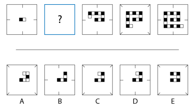
17) The answer is C. The patterns progress by adding two “building blocks” at a time in an outwardly spiraling form, where each building block comprises one black square followed by one white square. Furthermore, and more subtly, the tick marks alternate between the centers of the outer edges of the confining square and the corners of that square. Only answer C appropriately fills both patterns.
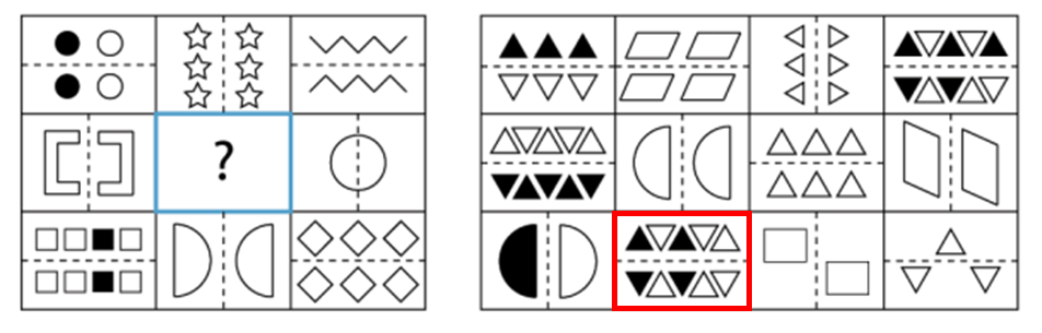
18) Each frame in the left-hand grid contains a set of shapes that are mirror-reflected without any change in black vs. white color. The mirror line alternates between horizontal and vertical orientation. The frame containing the question mark thus needs a mirror reflection of shapes about a horizontal line, with no change in color of the shapes. The mirror reflection implies, for example, that triangles or trapezoids are turned upside down in the reflected image. The only option in the right-hand grid that fits this description is bordered by a red square in Fig. 3 below.
19) The pattern established in the first three triangles is that the number inside the triangle is equal to (top number – lower left number) x lower right number. To complete the pattern, the missing number in the 4th triangle is 3, as indicated in Fig. 4 below.
VII. algebraic reasoning
20) This problem could be solved by trial and error, but it is straightforward with a little algebra. Denote the number of apples the prince initially picked by N. At each of the three troll stops, he had to surrender half of his remaining apples, plus two more. The number he retained after each troll stop is then summarized in the table below.
| Station | Number of Apples Prince Retains | Numerical Value |
| Start | N | ? |
| After 1st troll | [(N/2) – 2] | ? |
| After 2nd troll | {[(N/2) – 2]/2} – 2 = [(N/4) – 3] | ? |
| After 3rd troll | {[(N/4) – 3]/2} – 2 = [(N/8) – (7/2)] | 2 |
The last line of the table gives us an equation to solve: [(N/8) – (7/2)] = 2, implying
N = 8 x [2 + (7/2)] = 44.
Thus, the prince picked 44 golden apples, had 20 left after the first troll, 8 left after the 2nd troll, and 2 left after the final troll.
21) When presented with an apparently daunting problem, try to break it down into bite-size pieces that can be solved in succession. Here, imagine dividing 100 by 11 (getting 9, with a remainder of 1) a hundred times in succession. You don’t have to perform a hundred steps, because the pattern becomes clear pretty quickly, as suggested by the following set of equations:
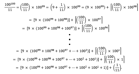
You don’t need to worry about evaluating the ugly expression inside the first set of square brackets in the last equation; you only need to recognize that it is a very large integer. The numerator in the final fraction inside parentheses in that last equation represents the remainder = 1.
VIII. order of magnitude estimates
22) The approach to these Fermi questions is again to break each issue down into bite-size chunks for which you can use everyday knowledge to make reasonable guesses. The precise values you estimate are less important than the thought process you go through in making your estimate. I’ll try to outline my thinking for each part.
How many golf balls can fit in a school bus?
Try to estimate the interior volume of a typical school bus and divide by the volume of a golf ball. A school bus might have 16 rows of seats, each taking up about 2.5 feet of length. Space for the driver would be equivalent to about two more rows. Thus, interior length might be about 45 feet. Interior height is about 6 feet and width about 10 feet. Then, total interior volume would be about 2700 cubic feet. Let’s allow about 10-15% of that volume to be already occupied by the seats themselves, so call available volume 2400 cubic feet. One cubic foot is equivalent to 123=1728 cubic inches. So available volume is roughly 4 million cubic inches. A golf ball might be about 2 inches in diameter. So let’s allot a cubic space 2 inches on a side to each ball, thus requiring a volume of 23=8 cubic inches. Dividing 4 million cubic inches of total available volume by 8 cubic inches allotted to each ball, you get roughly 500,000 golf balls to fill a school bus. There is no precise “right answer” here, but a sensible estimate should give several hundred thousand balls.
b) What is the weight of a large (e.g., Boeing 767) commercial airplane?
We can again try to estimate the total volume of the airplane, and then multiply by a guess at its average density to estimate total weight. A large commercial plane (think Boeing 747) might have about 50 rows of seats, each taking up about 3 feet of length on average. Add to this total length another 20% to accommodate the cockpit, rest rooms, and preparation areas for flight attendants. So let’s estimate body length at 180 feet, extending to about 200 feet when allowing for the plane’s tail. The interior width of a large plane typically includes 8 passenger seats and two aisles per row. Allowing 2 feet of width per seat and per aisle, that gives roughly 20 feet of width. Since the body of the plane is very roughly cylindrical, let’s take 20 feet as the diameter, or 10 feet as the radius r of the plane’s body (including luggage and landing wheel compartments and plane body, in addition to interior passenger space). We then estimate total volume of the plane’s body (apart from wings) to be pi r2 x length or about 60,000 cubic feet, of which maybe 90% is air-filled when the plane is empty of passengers, crew, luggage and fuel. Let’s guess that the average density of the solid materials making up the plane’s body, interior structures, seats, etc., is roughly twice the density of water, or 2 grams per cubic centimeter (we’re going to have to do some unit conversions here!). Then the average density of the entire volume, after we average in the 90% that is air-filled and of negligible density, is 10% of that, or 0.2 grams per cubic centimeter. There are about 30 centimeters in a foot, so one cubic foot is equivalent to 303 = 27,000 cubic centimeters. There are 1000 grams in a kilogram. So a rough estimate of the body weight (we will have to add wings after this) is (60,000 cubic feet) x (27,000 cubic centimeters per cubic foot) x (0.2 grams per cubic centimeter) x (1 kilogram per 1000 grams) or approximately 320,000 kg (700,000 pounds). The two wings have higher density, but a combined volume which is perhaps only 5% of the full body’s volume, so they add about 10% to the weight. Roughly, then, we might guess a total weight around 350,000 kg, or 770,000 pounds, or 385 tons. (Looking up, after our guesstimate, the actual weight of a Boeing 747 empty of passengers, crew and fuel, we find 220,000 kg, so our estimate is a little bit high, but still of the correct order of magnitude.)
c) How much heavier (i.e., by what factor) is a full-grown elephant than a full-grown mouse?
Assume that the density of matter in the elephant and in the mouse is about the same, since most of the body mass has the density of water, just as in humans. Then the ratio of weights is approximately equal to the ratio of volumes. A typical mouse might be 2 inches, or 5 centimeters, long, about 2.5 centimeters wide and 2.5 centimeters high. Its volume is thus, very roughly, about 30 cubic centimeters. At the density of water, that would correspond to a typical mass of 30 grams. Let’s estimate the height of a full-grown standing elephant as 10 feet, or about 300 centimeters, half of which is in its legs. We estimate its body length also as 300 centimeters, and its body width as 3 feet, or 90 centimeters. The volume of its body would then be approximately 150 x 300 x 90, or roughly 4 million cubic centimeters. In addition, there are 4 legs, each of which we can consider to be cylinders 150 centimeters high and 20 centimeters in diameter, or 10 centimeters in radius. So the legs add about 4 x 150 x pi x 100, or roughly 0.2 million cubic centimeters. Again, at the density of water, that total volume estimate of 4.2 million cubic centimeters corresponds to a mass of 4200 kilograms, or roughly 4 tons. In all, then, we estimate the ratio of weights to be of order 4.2 million cubic centimeters/30 cubic centimeters ~ 140,000. Again, only the order of magnitude really matters in this guesstimate.
23) There are approximately 330 million people in the U.S., so let’s estimate 150 million households. Let’s guess that 10% of these households, so about 15 million, are supported by food stamps. For the food stamps to be of use, they should probably provide for about $40/week or roughly $2000/year, which doesn’t buy all that many groceries. 15 million households receiving $2000/year would indicate an annual SNAP outlay of 30 billion dollars. (The total SNAP budget would be considerably higher, when one adds in salaries for its administration throughout the country.) So, the alleged waste of $70 million corresponds to about 0.2% of fraudulent waste. That is a valid argument for trying to find and eliminate the fraud, but hardly a compelling argument for eliminating the program. Many U.S. government expenditures involve much more than 0.2% waste. (A Google search after the estimate reveals that the annual food assistance program budget for 2018 was $68 billion.)
IX. identifying flawed probability arguments
24) The assumption that the probability of finding two or more individuals with the same birthday varies linearly with the number of people in the group is unjustified. It is not hard to estimate the probability of finding at least two individuals with the same birthday in a gathering. The alternative is that there are no common birthdays within the group. Let’s ignore leap-year birthdays on Feb. 29. Then the probability that a second person in the group has a different birthday than the first person is 364/365. The probability that the third person has different birthdays than either of the first two people is 363/365, and so forth, until the probability that the 37th individual has a different birthday than any of the previous 36 is (365-36)/365 = 329/365. Assuming that the group members are randomly selected, their birthdays are not correlated in any way. Then the total probability of having no shared birthdays among 37 randomly selected individuals is:
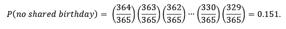
If there is only 15% probability of having no shared birthdays, that implies there is an 85% probability of finding at least two people with the same birthday among 37 randomly selected individuals.
25) Once you have chosen door #1, the host has two options for which other door to open to reveal a goat. If the car was actually behind your chosen door #1, the host could have opened either door #2 or #3 with equal probability. Thus, his choice of #3 comes with a 50% probability. If the car is actually behind door #2, he could only have opened door #3, so his choice comes with 100% probability in that case. Thus, the probability that the host would choose door #3 to open to reveal a goat is twice as large if the car is behind door #2 than if the car is behind your chosen door #1. The odds suggest that you should take the host up on the offer to switch your selection!
26) If the chance of a random false positive match is only 1 in 10,000, that implies that the probability that a randomly selected man would not match the crime scene DNA is 0.9999. But a search was made through a database containing 20,000 men. The probability that not even a single man in the database would match the crime scene DNA is then:
Thus, the probability of finding at least one false positive match among a database of 20,000 is 86.5%. The prosecutor’s argument is deeply flawed!
X. distinguishing random from non-random patterns
27) The correct answer is that option (a) is non-random. But let’s explore why. On any one coin flip there are two possible outcomes. For 54 uncorrelated consecutive flips, there are a total of 254 possible outcomes. Each of the four sets of results in the problem statement has the same probability of occurrence, namely 1/(254). So that’s not an effective way to search for non-randomness. You could try counting the number of heads vs. tails in each set. You would expect about half heads and half tails, so 27 of each. But there is a statistical uncertainty of ±5 on that result, so you should hardly be surprised to find individual results with anywhere from 22 to 32 heads, and only mildly surprised to find even 17 or 37 heads. The number of heads in each option is: (a) 16, (b) 28, (c) 30, (d) 27. From that point of view, option (a) looks suspicious, but can’t yet be ruled out definitively.
Each of the four sets involves clusters of heads or tails, and such clusters are normal in a random selection. But option (a) appears to have too many clusters of excessive length. The real distinguishing factor, however, is that option (a) has a clear pattern that is highly unlikely to show up in a random selection. The final 27 coin flips in option (a) exactly repeat the first 27 coin flip results. The eagle-eyed among you may notice the explicit pattern of repeats in option (a): 1-4-2-8-5-7-1-4-2-8-5-7. That exactly reflects the order of digits beyond the decimal point in the evaluation of the fraction 1/7 = 0.142857142857…. . That is the highly non-random algorithm used to generate the results in option (a)!
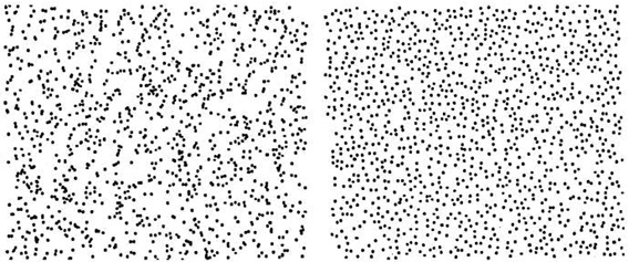
28) The right-hand star map in Fig. 5 is the non-random one, because it shows insufficient clustering. There are roughly 2000 dots in each map. If you were to divide the total space in each into 2000 equally sized pixels, you would expect to find an average of one dot per pixel. But statistical fluctuations about that average follow so-called Poisson statistics for a random distribution. For an average density of 1 dot per pixel, Poisson statistics indicate that we should expect to find pixels with zero dots 37% of the time, with one dot 37% of the time, with two dots 18% of the time, and with more than 2 dots 8% of the time. The right-hand map would include far fewer than 26% of pixels having two or more dots and far fewer than 37% having zero dots. The right-hand distribution is therefore highly unlikely to be random. In fact, it is based on the pattern of glow worms on the ceiling of the Waitomo caves in New Zealand. The glow worms keep their distance from one another in order that each has sufficient food in their immediate vicinity to survive on. You may think you see “constellations” in the left-hand plot, but that’s only because the human mind has evolved to perceive patterns, even where they may not really exist.
29) The grids in this problem are sort of colored versions of the star maps of problem #28. The upper right-hand grid in Fig. 6 is the non-random one, again because it displays too little clustering. In particular, no colors are repeated within any row, any column, or any of the nine 3 x 3 sub-grids into which the overall grid could be subdivided. That upper right grid is, in fact, a 1-9 sudoku puzzle interpreted in colors.
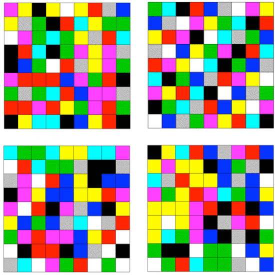
To make the analysis more quantitative, note that the probability of finding a single row or column of 9 squares with no repeat colors out of a random choice of 9 different colors is given by:

In fact, in the three random grids above, there is not a single row or column without repeated colors. The probability of seeing 9 distinct and uncorrelated rows, each without repeated colors, is:

that is, less than one part per billion billion billion. And this doesn’t yet take into account the additional tiny factors from demanding no color repeats in any column or subgrid. Thus, the upper right grid has negligibly small probability of occurring randomly.
30) We can examine the four draws to see if they meet random expectations for the distribution of cards among the four suits and the 13 denominations (ace through king). Among 20 cards, we should expect an average of 5 cards per suit. But with statistical fluctuations, we shouldn’t be surprised to see anywhere from 3 to 7 cards per suit. Each of the four draws satisfies this constraint. We should also expect to see 1 or 2 cards of each denomination, but again shouldn’t be surprised to see a denomination occasionally that has zero or 3 or even 4 cards. Draws (a), (b) and (d) satisfy this constraint, noting that draw (d) has zero 3-cards. The non-random draw (c) spectacularly fails this constraint, as it offers zero cards with 6, 7, 8, 9 or jack denominations. Those five denominations account for 40 of the 104 cards in the two combined decks. For all of them to be missing, each of the 20 cards must be drawn from the remaining 64 cards. The probability of this occurring at random is given by:

Thus, the probability of this occurring at random is only 15 parts per million. In fact, the algorithm used to generate draw (c) was to select cards at random from two decks with all 6’s, 7’s, 8’s and 9’s removed. The absence of jacks in that particular draw occurred at random.
