
January 3, 2026
I: IntroductioN
The earliest human written records date to about 3500 BCE, when the Sumerians developed cuneiform as a pictographic language useful for record-keeping and administration in early human societies. The independently developed Egyptian hieroglyphics entered the record several centuries later. Hence, human history has been recorded in some form for about 5,500 years, i.e., for almost the entire history of Earth according to the Judaeo-Christian Bible. But we know scientifically that homo sapiens have been around on Earth for more than 200,000 years, while the Earth itself is about 4.5 billion years old and our universe is close to 14 billion years old.
Human curiosity extends much further back in time than recorded human history or even human existence. Questions about how we got here have attracted great attention among scientists, religious leaders, archaeologists, paleontologists, and even some historians. We have been aware for many years that the distant past has left us clues in the form of architectural ruins, fossils, ancient human remains, geological strata, light from distant stars, and even a telltale background glow that originated in the universe long before any stars were formed. But only with technology developed over the past half-century have scientists begun to interpret those clues in ways that provide precise, quantitative information about our origins.
In this post we will review the quantitative analysis of clues from the distant past using three distinct approaches. The first, outlined in Section II, focuses on measuring and calibrating the abundances of long-lived radioactive isotopes in prehistoric artifacts to allow accurate dating. These analyses have led to major revisions to earlier narratives about how human civilizations first sprung up and have allowed scientists to illuminate current climate concerns with information about how ocean currents changed in ancient times.
The second approach discussed in Section III extracts and analyzes DNA from ancient human remains. When samples are extracted from enough individual ancient humans, scientists can begin to build a DNA database akin to that collected with modern 23andMe genetic testing. Such a database tells us, for example, where modern Europeans originated genetically in prehistoric times, revealing migration and fertilization patterns for ancient humans.
The third approach provided in Section IV involves high-precision measurements of the Cosmic Microwave Background radiation, a pervasive afterglow that originated some 380,000 years after the Big Bang that spawned our universe. The analysis of those measurements has determined the age and energy breakdown of the universe, as well as the distribution of matter in the early universe, with greater precision than anyone could have imagined a few decades ago. A new generation of such measurements carry the potential to illuminate the universe at an even earlier stage of its infancy, when theorists have proposed that the universe expanded at mind-blowing rates.
These examples from distinct fields of study illustrate the incredible creativity scientists have used to shed more light on just how we got here.
II: Radiometric Dating Revolutionizes Archaeology
The use of unstable isotopes has proved to be a powerful tool for scientific dating purposes. In this chapter we will discuss the method of radiocarbon dating and its applications to the field of archaeology. At the end of this section, we will describe how measurements of decay products of uranium can be used to study the time history of major ocean currents.
A: Radiocarbon Dating:
Radiocarbon dating was developed in the late 1940s by University of Chicago professor Willard Libby. There are three isotopes of Carbon that occur in nature: Carbon-12 (with six protons and six neutrons in its nucleus); Carbon-13 (with six protons and seven neutrons); and Carbon-14 (six protons and eight neutrons). While Carbon-12 and Carbon-13 are stable, Carbon-14 is unstable and undergoes radioactive decay. Libby noted that Carbon-14 or 14C is being created in the atmosphere from neutrons that are present in cosmic rays. A neutron interacts with the nucleus of nitrogen-14, the most abundant element in the atmosphere, creating carbon-14 plus a proton; the equation is
n + 14N –> p + 14C (1)
Since Carbon-14 is unstable, it decays into Nitrogen-14 plus an electron plus an antineutrino, through the process

In the atmosphere, the process is in equilibrium; the rate at which C-14 is produced is equal to the rate at which it decays. Thus, the ratio of Carbon-14 to Carbon-12 in the atmosphere is relatively constant (we will discuss exceptions to this later). In the atmosphere, there are roughly 1.25 atoms of C-14 to every trillion atoms of C-12. Carbon-14 has exactly the same chemical properties as the most common stable isotope Carbon-12. Thus, C-14 is found in molecules of carbon dioxide in the atmosphere. Living plants exchange carbon dioxide with the atmosphere and thus obtain some C-14, and animals eating the plants also ingest C-14. When they are alive, plants and animals will have the same ratio of C-14 to C-12 as the atmosphere. When the plants and animals die, they no longer take in any C-14; thus, the C-14 decays and the ratio of C-14 to C-12 decreases over time. Knowing the rate at which C-14 decays and measuring the C-14/C-12 ratio in formerly living specimens, one can determine the length of time since the specimen died.
The current best experimental value for the half-life of Carbon-14 is 5,700 ± 30 years. Carbon-14 decays exponentially, as shown in Figure II.1. So after 5,700 years a sample of plant or animal matter will have half as many Carbon-14 nuclei as the sample when it was alive. Typically, one measures the rate at which electrons from C-14 decay are being emitted from the sample and compares that with the rate that Carbon-14 decay electrons were being emitted from the sample when it was alive. If, for example, the sample was 5,700 years old, the rate of electron emission per unit mass will be half the rate from a living sample; if the sample is 11,400 years old (two half-lives), then the rate of electron emission will be one-fourth of that from the living sample. After 57,000 years, less than 0.1% of the original C-14 will remain. At this point, there will be such small amounts of Carbon-14 left in a sample that Radiocarbon dating cannot be reliably used to date the object.
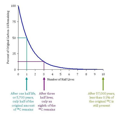
Figure II.1. A diagram showing the exponential rate of decay of carbon-14. The “half life” of C-14 is 5,700 years. Thus, after 5,700 years one half of a sample of C-14 will have decayed. After three half-lives (17,100 years), only one-eighth of the C-14 remains.
In 1949, Libby and James Arnold published a test of carbon dating methods. They compared results they obtained for the age of samples taken from the tombs of two Egyptian kings, for which the dates were known from independent methods. While the known sample dates were 2625 BCE ± 75 years, the radiocarbon dating methods gave an average of 2800 BCE ± 250 years. It became immediately clear that radiocarbon dating techniques could be used to obtain the age of ancient samples containing organic material. In some cases ages from antiquity had been estimated by other means, and in other cases the ages were unknown. Within 11 years of the Libby-Arnold paper, more than 20 laboratories had been established worldwide to utilize these techniques; and in 1960, Willard Libby was awarded the Nobel Prize in Chemistry, “for his method to use carbon-14 for age determination in archaeology, geology, geophysics, and other branches of science.”
Radiocarbon dating has been used extensively to measure the age of ancient objects. One of the most famous uses of radiocarbon dating has been to study the Dead Sea Scrolls. This refers to a collection of nearly 1,000 texts and fragments, many of which were discovered during the period 1946 to 1956 near the area of Qumran, which is close to the Dead Sea. Figure II.2 shows a page of one of the Dead Sea Scrolls. Carbon-14 dating of various scrolls at the Accelerator Mass Spectrometry (AMS) Lab of the Zurich Institute of Technology in 1991, and later at the AMS Lab at the University of Arizona in 1994-1995 found that they were produced between 385 BCE (Before Common Era) and 82 CE (Common Era), with an accuracy rate of 68%. The same scrolls were analyzed using paleographic methods, where scholars used the size, variability and style of the writing to estimate the age of the scrolls. The paleographic methods gave dates for the scrolls from 225 BCE to 50 CE. Thus, these two methods of analysis gave comparable dates for the scrolls.
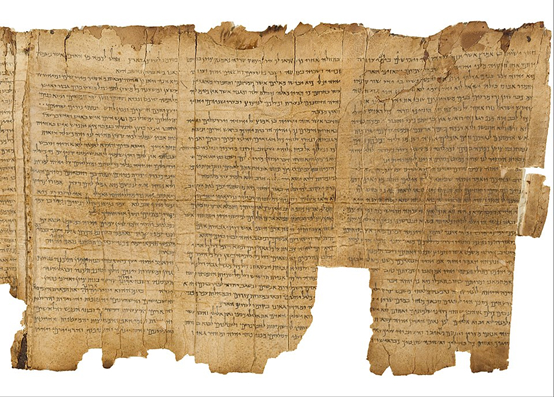
Figure II.2: A fragment of one of the Dead Sea Scrolls that were discovered between 1946 and 1956 on the northern shores of the Dead Sea in Israel. Carbon dating techniques were used to verify the authenticity of the scrolls and to determine when they were written.
B: Assumptions and Details of Radiocarbon Dating:
In order to make precise dating determinations, one has to consider the assumptions in greater detail. For this section, we will only treat land-based organisms. Marine life obtains its carbon from the oceans; in this case there are many details regarding the distribution of carbon in the oceans, effects that take place at or near the ocean surface, and other considerations that are too detailed for this summary.
A major aspect of radiocarbon dating is the half-life for Carbon-14 decay. This has varied somewhat over the years as we will discuss; for a while after Libby’s first measurements, the best value for the half-life was 5,568 years. Measurements taken before the current value of 5,700 ± 30 years need to be corrected, and correlation tables have been created to make these adjustments.
Another assumption in radiocarbon dating is that the proportion of Carbon-14 is the same in all living organisms. But there are corrections that need to be made in certain circumstances. One of these effects arises from the mass difference between C-12 and C-14. This is called isotopic fractionation. In photosynthesis, carbon dioxide containing Carbon-12 is absorbed slightly more easily than molecules with Carbon-13 or Carbon-14. The rate of isotopic fractionation varies for different substances. To determine fractionation in various organisms, researchers look at variations in the C-13 to C-12 ratio in a substance, compared to their ratio in the atmosphere. This is relatively easy to do since in the atmosphere C-13 accounts for about 1% of carbon content. Once researchers determine the magnitude of the mass effect for Carbon-13, they double it since C-14 has two additional neutrons while C-13 has one.
Another assumption is that at any given time, the atmospheric C-14/C-12 ratio is the same all over the world. It is now known that this ratio depends on several atmospheric effects. We will mention one of these, called the hemispheric effect. This arises because the area of the ocean in the Southern Hemisphere is substantially greater than in the Northern Hemisphere. Thus, there is more Carbon exchanged between the atmosphere and the ocean in the Southern Hemisphere. The surface of the ocean is depleted of C-14; as a result, more Carbon-14 is removed from the Southern Hemisphere atmosphere. This requires a correction when using radiocarbon dating techniques on Southern Hemisphere organisms.
Time Variation of C-14 Abundance:
Radiocarbon dating initially relied on the assumption that the ratio of C-14 to C-12 in the atmosphere had remained constant over the years. However, it turns out that the ratio of C-14 to C-12 has varied substantially over the years. We will discuss two of these effects: increases in the amount of C-14 in the atmosphere arising from atmospheric nuclear weapons testing; and increases in the amount of C-12 due to the burning of fossil fuels.
A significant variation of the atmospheric abundance of Carbon-14 occurred during the period 1950 – 1963, when various countries including the U.S., U.S.S.R., and Britain were undergoing nuclear weapons tests in the atmosphere. Explosion of an atomic or hydrogen bomb produced a vast number of neutrons. These neutrons could combine with 14N in the atmosphere to produce 14C via the procedure of Eq. (1). Therefore, during the period of atmospheric testing of nuclear weapons, the amount of 14C in the atmosphere increased greatly. Figure II.3 shows the percentage increase of atmospheric 14C as a function of time. The blue curve shows the average increase in C-14 in the Northern hemisphere, while the red curve shows the average increase in the Southern hemisphere. The percent increase begins in about 1956 and reaches a peak in 1963, when the increase in atmospheric C-14 reaches almost 80% in the Northern hemisphere. The Partial Test Ban Treaty went into effect in October 1963. That treaty was signed by 126 countries, plus another 10 countries that signed the agreement but did not ratify it. The agreement banned nuclear weapon tests in the atmosphere, in outer space or under water. Non-signatory nations France and China continued above-ground nuclear weapon tests until 1980, and signatory nations Israel and South Africa may have detonated a nuclear weapon in 1979; however, since that time all nuclear weapons tests (including nuclear detonations by India and Pakistan in 1998) have been underground.

Figure II.3: Increase of C-14 in the atmosphere, in percent, vs. time, between 1950 and 2010. Atmospheric nuclear weapons explosions occurred during the period 1950 – 1963, after which such atmospheric tests were banned. Blue curve: average percent increase of C-14 in the Northern hemisphere; red curve: average increase in the Southern hemisphere.
Another cause of major variation of Carbon isotopic ratios in the atmosphere arises from the burning of fossil fuels. Figure II.4 shows the increase of carbon dioxide in the atmosphere from 1751 to 2024 (in parts per million: blue curve and left axis). Until the beginning of the Industrial Revolution, atmospheric CO2 levels were about 280 parts per million. But carbon dioxide levels began rising around 1850 at the beginning of the Industrial Revolution. Burning of fossil fuels produces large amounts of carbon dioxide, much of which enters the atmosphere. The black curve and right axis shows annual CO2 emissions over time. There are essentially zero carbon dioxide emissions until about 1860. Since the fossil fuels are derived from organic material that died millions of years ago, the 14C in them has long since decayed. So, added carbon dioxide in the atmosphere arising from fossil fuel burning lowers the 14C/12C ratio. Over the past 175 years, carbon dioxide from fossil fuel burning has increased the CO2 in the atmosphere by 50% to its current value of about 430 ppm. This is a second source of change in the 14C/12C ratio over time.
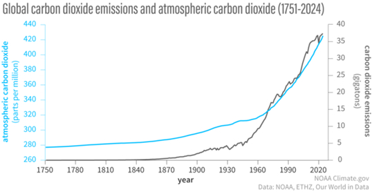
Figure II.4: The amount of carbon dioxide in the atmosphere vs. time, from 1751 to 2024 (blue curve and left axis, in parts per million). Also, annual emissions of carbon dioxide over time (black curve and right axis, in gigatons). Carbon dioxide levels in the atmosphere have increased by 50% since the beginning of the Industrial Revolution. This increase in CO2 over this period is almost entirely due to burning of fossil fuels.
Dendrochronology:
Dendrochronology, or the study of tree rings to produce time sequences, has been of great help in providing a firm basis for radiocarbon dating. As trees grow, every year they tend to produce new wood that forms around the existing trunk. Figure II.5 shows a cross-section of a tree trunk, showing the annual growth rings that form. The newest rings are those closest to the bark of the tree. For the purposes of dendrochronology, the most useful trees are those in the temperate zone that, under normal circumstances, produce one ring per year. Each ring then marks one year’s cycle of growth in the tree’s life.
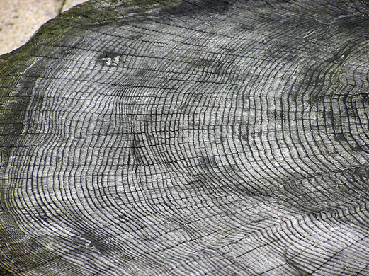
Figure II.5: The annual growth rings of a tree at the Bristol Zoo in England. A ring is produced every year. The outside rings nearest the bark are the youngest.
The most useful trees for the purpose of dendrochronology are those that live the longest. For this purpose the bristlecone pine which grows in the American Southwest is useful because of its exceptionally long life span. The longest-lived specimens of bristlecone pines, found in the White Mountains of California, have been dated at nearly 4,900 years old. Figure II.6 shows a bristlecone pine from the White Mountains. One can use long-lived trees to obtain a timeline of their annual rings. One can then compare living specimens with dead trees, to create an unbroken time sequence that goes back even further. The great utility of tree ring analysis is that each ring contains carbon that was assimilated in the year the ring was formed. Thus, analyzing the level of Carbon-14 in a given tree ring determines the atmospheric C-14 in that year. This has been done with living and dead bristlecone pines and we now have a timeline of C-14 abundances going back about 11,000 years. In addition, we now have tree-ring data, primarily from oak trees, from countries like Germany and Ireland where dating can encompass 13,910 years.

Figure II.6: A bristlecone pine in the White Mountains of California. These are the longest-lived known trees. One of the trees in a grove there is aged nearly 4,900 years.
C: Radiocarbon Dating Revolutionizes Archaeology:
The introduction of calibrated radiocarbon dating put the dating of artifacts on a firm scientific footing. Before carbon dating techniques were available (which gives an accurate age for organic artifacts up to about 60,000 years old), archaeologists had to rely on comparative analysis of artifacts in different cultures. As we will see, these analyses involved assumptions about the capability of various cultures. Prior to scientific evidence from carbon dating, many researchers implicitly assumed that “primitive” societies were incapable of discovering advanced techniques on their own. The only way that barbarian societies could develop these techniques would be either direct contact with travelers from more advanced cultures, or through introduction to modern techniques by obtaining artifacts from societies who had mastered these skills. This line of reasoning is known as the diffusionist theory. Until calibrated carbon dating was applied to archaeological sites, diffusionism was the dominant paradigm in archaeology.
Here, we will discuss the diffusionist approach to archaeology. We will then examine the great monumental site at Stonehenge in England. We will discuss two central questions regarding that monument: when was it built? And what was its purpose? We will review diffusionist arguments regarding that structure, and we will show how many conclusions from the diffusion hypothesis were completely demolished once the Stonehenge structure was subjected to calibrated C-14 dating.
Theory of Diffusion in Archaeology:
The field of archaeology deals with an understanding of the ancient world. In particular, one used meticulous studies of artifacts to establish the dates associated with various cultures. However, before the advent of written records in ‘primitive’ societies, it was extremely difficult to establish when various events had occurred. In the 17th Century, one guide was to use religious myths to provide timelines for events. For example, Archbishop Ussher famously used events and genealogies described in the Bible to determine the date for the Creation of the world as 4004 BCE. Ussher’s calculations allowed Sir Isaac Newton to criticize the chronology claimed by the Egyptians. He noted that records of Egyptian kingdoms extended back before 5000 BCE. Newton scoffed at the Egyptian claims, as “Out of vanity [they]have made this monarchy some thousands of years older than the world.”
Eventually, one could make educated guesses regarding the times of ancient events by using geological data and the assumption that these processes had unfolded at the same rates that we observe today. But until methods like radiocarbon dating evolved, the best estimates for the age of Western European events were to date them relative to the oldest reliable records from other cultures. These would be records of the Egyptian kingdoms, which went back to about 3,000 BCE, and those of the Sumerians whose records extended well before 2,000 BCE.
Archaeologists proposed timelines of ancient people with no written records into three different ages, based on where various artifacts were discovered in geological strata. The first of these was the Stone Age, which was subdivided into an older (paleolithic) era and a newer (neolithic) era. Instruments typical of the paleolithic era were chipped stone tools, while polished stone axes were characteristic of the neolithic era. More recent eras such as the Bronze age and the Iron age were marked by discoveries of implements made from these respective metals. However, although this allowed archaeologists to determine which were the earlier and the later eras, it did not provide absolute time scales for these time periods.
One of the first solid steps towards an absolute chronology of European cultures was obtained by Sir Flinders Petrie, a noted Egyptologist. In excavating pottery at a site in Kahun, Egypt, Petrie found samples that had originated in Crete. Those samples could be dated around 1900 BCE, and hence contacts between the two cultures had commenced at least that early. Petrie then traveled to Mycenae, on the Greek mainland, and found Egyptian imports that he could date fairly accurately to about 1500 BCE. Combining the direct evidence of contact between two cultures with more recent evidence from both artifacts and radiocarbon dating, we can now set the beginning of the Early Minoan culture in Crete at about 3000 BCE.
But for other European cultures, there was little direct evidence of trading with people from Egypt or Greece. Therefore, most archaeologists used a diffusion model to explain similarities between European artifacts (from megalithic burial chambers to hand axes and daggers) and those from Egypt or from the Orient. The Swedish archaeologist Oscar Montelius was a major figure advocating for the diffusion model. For Montelius, it seemed obvious that western European culture resulted from the diffusion of ideas and practices from Egypt and the Orient. Montelius explained, “At a time when the people of Europe were, so to speak, without any civilization whatsoever, the Orient, and particularly the Euphrates region and the Nile valley, were in enjoyment of a flourishing culture … The civilization which gradually dawned on our continent was for long only a pale reflection of Oriental culture.”
The diffusion model was a great help in assigning timelines for European cultures. Since all of western Europe’s civilization was supposed to have originated earlier in Egypt, Greece, and the Middle East, once one established dates for the advent of Bronze Age metallurgy in Aegean societies, then similar practices in, say, France would of necessity have to be later, to allow for diffusion of these skills to the West. Now that radiocarbon dating has invalidated much of the diffusionist dating methods, we can look back and see the extent to which these arguments were based on specious reasoning regarding ancient cultures. Many of the archaeologists who were active before 1950, when carbon dating was first applied to archaeological sites, were motivated by implicit biases regarding the superiority of Egyptian and Greek societies. In several cases, these researchers expressed their confidence that at a time when impressive Egyptian and Greek cultures were flourishing, western Europeans were “mere barbarians” who were “without any civilization whatsoever.” The lack of French pyramids or English temples, and the lack of written records seemed to justify the beliefs of archaeologists that any structures found in western Europe must have diffused from superior cultures in Egypt or Greece. Any similarities found, or in some cases imagined, in structures found in western Europe were assumed to have originated in these earlier cultures. As we will see in the next section, many of these claims were eventually firmly contradicted by radiocarbon dating, which provided precise independent dates for the origins of western European artifacts.
Diffusion models of cultural dissemination reached perhaps a peak in the work of Sir Grafton Elliot Smith, the Professor of Anatomy in Cairo in the 1920s. Smith convinced himself that all civilizations of the world, and indeed all human progress, were the result of traveling Egyptians, who carried their knowledge to people all over the world. This is depicted in a map produced by Elliot Smith, shown in Figure II.7, to illustrate the diffusion of knowledge around the world. Like many diffusionists, Elliot Smith believed that important breakthroughs in European culture were the result of diffusion of knowledge that originated in Egypt (although the quality of the map in Fig. II.7 is poor, all arrows in Elliot Smith’s map originate in Egypt), Greece or Mesopotamia. Many archaeologists believed that paleolithic structures and artifacts in western Europe resulted from those people becoming aware of the accomplishments from earlier societies. However, Elliot Smith was convinced that the dissemination of knowledge came directly from Egyptian explorers, or in his words “the Children of the Sun.” who traveled to distant lands and introduced the barbarians to knowledge created in Egypt. And unlike other diffusionist archaeologists, Elliot Smith extended the diffusion picture around the entire globe – according to him, traveling Egyptians inspired cultures in Australia and the Pacific, and after that to North and South America!
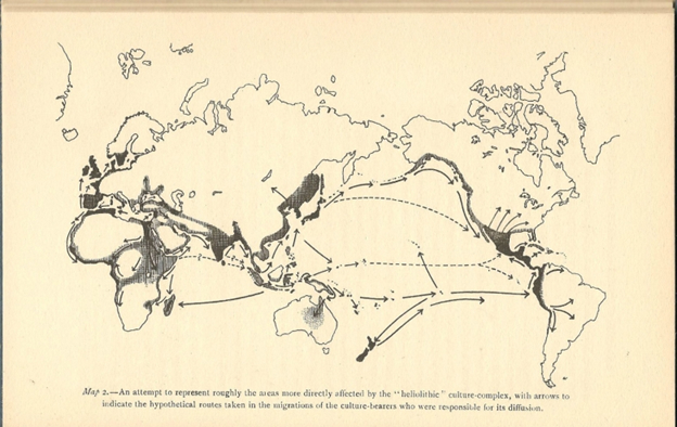
Figure II.7: Map by early 20th century archaeologist Grafton Elliot Smith showing his claims regarding the diffusion of knowledge around the world. In Smith’s view, all arrows initially originate in Egypt. Smith claimed that not only cultures in Europe and Asia, but also Australia and the Pacific Islands, and both North and South America, were inspired by Egyptians who traveled to those countries and imparted Egyptian technical knowledge to the barbarians there.
Another ardent diffusionist was Gustav Kosinna. In his theories, the origin of Western culture arose not in Egypt or Greece, but in an “Indo-Germanic” culture that spread all across Europe. So, Kosinna argued that writing was invented in Europe and diffused out from there, as did metallurgy. According to Kosinna’s nationalist worldview, “The Germans were a heroic people and have always remained so. For only a thoroughly manly and efficient people could have conquered the world at the end of the Roman empire … The great folk movements then went out, in the third millennium B.C., from north-central Europe … populating all Europe, and especially southern Europe and the Near East, with the people who speak our tongue, the language of the Indo-Germans. Everywhere people of central European blood became the ruling class … and imprinted at least our language, as an eternal symbol of the world-historical vocations of our race, indelibly upon those lands.” It is no coincidence that Kosinna’s nationalistic claims sound eerily like the Nazis and their mantra of “Aryan” supremacy. A later version of Kosinna’s book is filled with quotes from Hitler, and Heinrich Himmler was also a big fan of Kosinna’s arguments about prehistory. Kosinna’s work also dove-tailed with expansionist policies of the Third Reich: if ‘Germanic’ artifacts were found in another European country, then that country would have belonged to an earlier Germanic empire, and Nazis argued that the country should be part of the new Germany.
Some diffusionist ideas continued long after radiocarbon dating techniques should have quashed those theories. As late as 1970, explorer Thor Heyerdahl crossed the Atlantic in a papyrus reed boat, sailing from West Africa to Caribbean islands in order to “prove” his theory that the Egyptians could have sailed to South America and been responsible for Mesoamerican architecture. In the late 1940s Heyerdahl had earlier sailed from South America to Polynesia in order to “prove” his theory that Polynesia was first populated by fair-skinned, red-headed South Americans. Figure II.8 shows the raft Kon-Tiki that Heyerdahl built and sailed from South America to Polynesia. Heyerdahl’s inherently racist theories (he believed that Southeast Asians were unable to master long-distance sailing methods) contradict all known scientific evidence comparing these different societies. Nowadays archaeological, linguistic, cultural, and genetic evidence supports a western origin for Polynesians. In fact, the original Polynesians came from Southeast Asia and used sophisticated knowledge of winds and currents to make long-distance voyages in multi-hulled crafts.
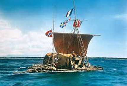
Figure II.8: The raft Kon-Tiki. In 1947, Thor Heyerdahl sailed this raft from South America to Polynesia to ‘prove’ his theory that Polynesia was settled by white South Americans before it was colonized by its current inhabitants. Heyerdahl’s theories are overwhelmingly rejected by all known scientific evidence.
Radiocarbon Dating and the Evolutionary Theory:
Very soon after Willard Libby announced the radiocarbon dating technique, that method was applied to ancient artifacts. However, early applications made systematic errors by assuming that the C-14/C-12 ratio in the atmosphere had been constant over time. For example, Libby’s initial use of radiocarbon dating for Stonehenge, carried out in 1952, dated the monument’s main stone phase to 1848 BCE. Later, after careful calibration of radiocarbon dating by comparison to tree rings, Stonehenge was determined to be significantly older. Colin Renfrew, in his book Before Civilization, refers to this calibration as the “radiocarbon revolution,” which rapidly overturned many existing archaeological claims. In particular, the claim that certain practices or artifacts must have ‘diffused’ from advanced cultures to primitive ones was often shown to be completely false. Today, myriad claims from diffusionist theories have been falsified by calibrated carbon dating. This is not the case with all diffusionist claims: there are cases where various advances occurred through direct contact between cultures, or when modern techniques were spread to less advanced societies. However, the advent of calibrated radiocarbon dating caused a real revolution in archaeology.
In this post we will use only a single example – the vast complex of Stonehenge in England – to illustrate how this structure and its people were viewed through the diffusion model, and how that model was completely invalidated once carbon dating techniques were applied to the site.
Stonehenge:
Stonehenge is a prehistoric megalithic structure located on Salisbury Plain in Wiltshire, England. As shown in Figure II.9, it consists of an outer ring of vertical sarsen standing stones. Each of these is about 4 meters high and 2.1 meters wide and weighs about 25 tons. Atop the standing stones are horizontal lintel stones; the lintel stones are held in place by mortise and tenon joints. Figure II.10 shows the mortise and tenon joints that connect the lintel stones, and the bumps and indentations by which the lintel stones are fixed onto the sarsen stones. The mortise and tenon joints are derived from woodworking techniques, although Stonehenge is the first known instance of this technique being used in a stone structure.
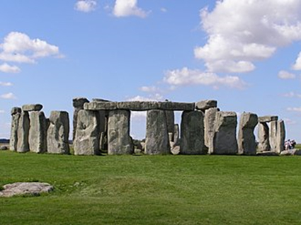
Figure II.9: A photo of Stonehenge, showing the vertical sarsen stones and the horizontal lintel stones.

Figure II.10: The lintel stones at top, showing the mortise and tenon grooves that hold those horizontal stones together. The lintel stones are connected to the vertical sarsen stones by bumps at the top of the sarsen stones that fit with semihemispheric indentations in the sarsen stones.
Figure II.11 shows a detailed diagram of the Stonehenge monument today. We have already discussed the outer ring of sarsen stones and lintel stones. There is an interior ring of smaller bluestones. Then there is a collection of trilithons, consisting of two vertical sarsen stones joined by a single lintel. There were five trilithons that formed a horseshoe shape within the bluestone circle, but only one of the trilithons is currently upright. Different colors in Figure II.11 denote sarsen stones, lintel stones, dolerite bluestones, and bluestones of other origin. Stone 56 (not labeled in Fig. II.11) is a large sandstone rock called the Altar Stone. It had apparently been brought to this monument from about 690 km away in northern Scotland. Another stone not shown in Figure II.11 is called the Heel Stone. It lies outside the sarsen circle to the northeast, along the monument axis noted in the figure. We will later discuss the astronomical significance of the monument and the Heel Stone.

Figure II.11: The Stonehenge monument today. The picture shows an outer ring of vertical sarsen stones each weighing about 25 tons with horizontal lintel stones connecting them. There is also an inner circle of smaller bluestones. Originally, there were five trilithons that formed a horseshoe inside the bluestone circle; each consisted of two sarsen stones connected by a lintel stone and paired with a bluestone.
The Stonehenge monument is a spectacular achievement. Archaeologists debated a number of questions about the monument and the people who erected it: in particular, when was Stonehenge erected, and what was the purpose of this imposing structure? In medieval times, the size of the edifice convinced some philosophers that the transportation and assembly of the stones had been accomplished through magical means by Merlin. Later, historians surmised that Stonehenge was inspired by the architecture of Roman temples; the notion that this monument owed its structure to the Romans seemed to be obvious: “What other culture would have had the knowledge to build such a structure?” Before radiocarbon dating, it seemed self-evident that earlier barbarian cultures could not have been sufficiently advanced to construct such a monument. According to this diffusionist reasoning, a Roman influence would have placed the construction of Stonehenge after about 500 BCE.
Radiocarbon dating and other archaeological studies have now provided precise dates for Stonehenge; and these studies have completely invalidated diffusionist arguments regarding the timeline of this monument. The site of Stonehenge appears to have once housed a series of large wooden posts that date back to about 8000 BCE. It is now believed that the community that built Stonehenge had occupied the site for several millennia before the large stone structures were assembled.
The Stonehenge monument was installed over a significant period of time, and in several stages, from about 3100 BCE to 1600 BCE. Furthermore, the stones were hauled to this site over very large distances; thus, the precise location of the monument was clearly very important. The sarsen stones are now known to have come from a quarry about 26 km north of Stonehenge. They were erected between about 2600 BCE and 2400 BCE. The interior circle of bluestones was installed during the period 2400 — 2200 BCE and came from a quarry in Wales about 260 km away. These dates establish that Stonehenge construction preceded that of the Roman temples that were once assumed to have inspired Stonehenge. The bluestones may have been used in an earlier structure and then carried to Stonehenge.
For a very long period of time, the Stonehenge vicinity was used as a burial site. Scientists have found many remains of burials in this region; and it is possible that the bluestones may have marked various grave sites. One remarkable feature of the monument is the presence of ancient carvings on sarsen stones in the trilithon horseshoe. Images of a Bronze age dagger and several axeheads have been found on these stones. It had long been assumed that these carvings were produced by quite recent vandals, until laser scanning of the carvings confirmed that they dated back to the late Bronze Age.
It is now known that one purpose of the Stonehenge monument was as an astronomical observatory. Figure II.12 shows directions of sunrise and sunset with respect to the orientation of Stonehenge. If the Heel Stone outside the Stonehenge circle (upper right-hand corner of Figure II.12) was upright, then at the summer solstice the Sun would have risen directly over that stone as observed from the center of the Stonehenge circle. This is confirmed in Figure II.13, which shows the Sun rising above the Heel Stone on the summer solstice. Rising of the Sun at the December winter solstice would have taken place at right angles to the summer solstice sunrise. Stonehenge lies at almost exactly the latitude where these relative directions of the summer and winter solstice would occur.
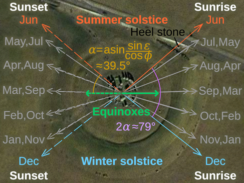
Figure II.12: Directions of sunrise and sunset with respect to the orientation of Stonehenge. If the Heel Stone outside the Stonehenge circle (in the upper right hand corner of this figure) was upright, then at the summer solstice the Sun would have risen directly over that stone as observed from the center of the Stonehenge circle. Rising of the Sun at the December winter solstice would have taken place at right angles to the summer solstice sunrise.
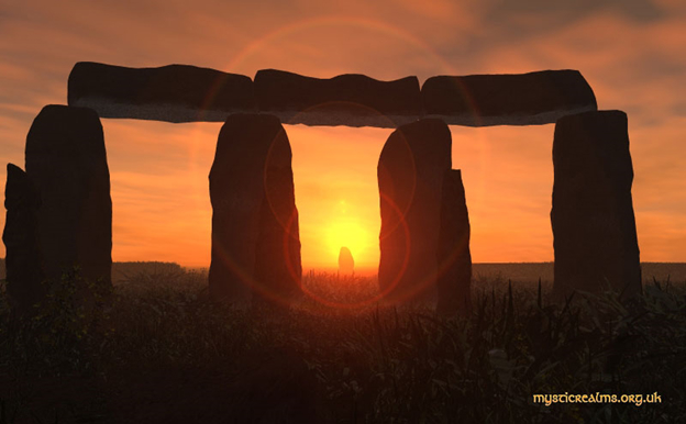
Figure II.13:The Sun rising over the Heel Stone in the background and shining through the central sarsen stones, as viewed from the center of the Stonehenge monument, on the Summer Solstice.
In a 1966 book titled Stonehenge Decoded, astronomer Gerald Hawkins argued that Stonehenge was a massive astronomical observatory. Hawkins discussed in detail the location and orientation of Stonehenge, and its probable use in determining summer and winter solstices. But Hawkins continued to argue that a series of holes called the Aubrey holes and some rectangular stones found at the site could have been used to predict lunar and solar eclipses. At the time Hawkins’ book was published, many archaeologists disagreed strongly with his claims. For example, historian Richard Atkinson critiqued Hawkins’ book as “tendentious, arrogant, slipshod, and unconvincing.” According to Atkinson, the people who built Stonehenge were “howling barbarians” — a familiar remark from an ardent diffusionist. It seems obvious to us that, at least regarding seasonal landmarks such as solstices and equinoxes, the location and orientation of Stonehenge has astronomical significance. Of course, it is also possible that the Stonehenge site was used in many other ways.
Radiocarbon dating techniques have become an essential tool in determining the dates when artifacts were created. Today, it would be unthinkable not to apply carbon dating to any archaeological site produced in the last 60,000 years. We showed that radiocarbon dating techniques demonstrated that Stonehenge was constructed far earlier than claimed by diffusionist researchers. There is no way that the monument was inspired by Roman architecture. It is now apparent that the “rude, uncivilized barbarians” in ancient England were able to design and construct a structure that could measure astronomically notable dates to exceptional precision. We now know of Mesoamerican sites that built structures achieving similar astronomical precision to Stonehenge. It now appears that monuments such as Stonehenge and Chichen Itza in the Yucatan must have evolved independently.
Indeed, in their 2021 book The Dawn of Everything, archaeologist David Wengrow and anthropologist David Graeber argue that modern archaeology overthrows much of what was previously believed about the development of human civilizations. For example, they argue that “Settlements inhabited by tens of thousands of people make their first appearance in human history around 6000 years ago, on almost every continent, at first in isolation,” each with their own specialty crops, domestic animals, and distinctive culture. The idea of independent evolution would be familiar to biologists, who frequently observe a feature called convergent evolution, where evolutionary pressures produce very similar results independently in different species. An example from biology would be the evolution of flight, which has evolved independently in birds, insects and bats.
Examining diffusionist arguments today, we are struck by the misplaced confidence of early archaeologists, who confidently argued that achievements of ‘primitive’ societies could only have arisen from the diffusion of knowledge from ‘superior’ cultures. Any similarities between these cultures were assumed to have flowed from the more ‘advanced’ group. Researchers who had studied the achievements of Egyptian, Greek or Mesopotamian cultures were so impressed by the advances of those cultures that they naturally assumed societies lacking written works could not possibly have independently erected precise astronomical sites such as Stonehenge. In the work of Kosinna and others, we also see elements of toxic nationalism that led to fields such as eugenics.
We mentioned that because of the half-life of C-14, radiocarbon dating can only be used to date artifacts that are 60,000 years old or less. In the next sub-section, we will discuss other methods that use isotopes with much longer half-lives to extend radioactive dating methods to study much older processes.
D: Other Examples of Radiometric Dating
Radiometric dating with naturally occurring unstable isotopes whose lifetimes are measured in the hundreds of millions or billions of years has been used to provide the best estimates of the age of our solar system. For example, potassium-40 decays with a half-life of 1.3 billion years; rubidium-87 decays with a half-life of 47 billion years. But some of the most useful dating has been done by tracing radioactive decay chains of uranium isotopes. Uranium-238, the most abundant isotope, decays through a long chain of alpha-particle emissions, ending at lead-206 with a half-life of 4.5 billion years. The decay chain of another isotope, uranium-235, ends at lead-207 with a half-life of 710 million years. The difference between these two half-lives has allowed the most precise dating of meteorites found on Earth, by measuring the ratio of lead-207 to lead-206 and comparing them to the naturally occurring abundances of these two isotopes determined from galena lead ores. Using this technique, the oldest meteorites found all have ages between 4.53 to 4.58 billion years, suggesting the age when our solar system began to form.
In our previous post on Climate Tipping Points, we have noted another unique dating exercise dependent on ratios of uranium decay daughter isotopes, which has illuminated the long history of a major Atlantic Ocean current that is now in danger of tipping from ongoing climate change. Thorium-230 (230Th) results from the decay of uranium-234, but is itself unstable and decays with a half-life of 75,000 years. Protactinium-231 (231Pa) results from the decay of uranium-235 and has its own half-life of 33,000 years. From naturally occurring uranium, which is distributed roughly uniformly throughout Earth’s oceans, the production ratio of these two daughter isotopes should be 231Pa/230Th = 0.093. Although uranium-235 is more naturally abundant than uranium-234, the probability of the former isotope’s decay to protactinium-231 is far smaller than that of uranium-234 to thorium-230.
Both of these uranium daughter isotopes eventually get adsorbed on marine particles in the ocean and deposited in sediment on the ocean floor. But because of their different chemistry they have different average time scales for doing so. Thorium-230 ends up in ocean sediment with a typical time scale of 20 years, while the more soluble protactinium-231 remains free in the ocean for a typical span of 130 years. The two isotopes are therefore transported southward by a major Atlantic Ocean current at quite different rates. The Atlantic Meridional Overturning Circulation, or AMOC, is a vast vertical circulatory pattern in which warm, salty seawater flows northward from the Southern Ocean along the surface, while the denser cold, salty water sinks to great depths in the North Atlantic and then flows southward far below the surface. When the AMOC flow is strong, as it is presently, that deep, cold current carries protactinium-231 southward at much greater rates than thorium-230, because the former isotope remains free in the ocean longer. The ratio 231Pa/230Th in North Atlantic sediment then falls well below its production value of 0.093. Today that ratio in the North Atlantic is about 0.055.
There are concerns from ongoing global warming that the accelerating melting of the Greenland Ice Sheet may at some point disrupt the AMOC because the flow of cold, fresh water from ice melt will mix with cold, salty water in the North Atlantic and interfere with it sinking. It is thus of great interest to determine whether the AMOC has collapsed during Earth’s paleoclimate history. We can now illuminate that question by measuring the 231Pa/230Th ratio in North Atlantic sediment samples that are independently dated by the measurement of other radioactive isotope ratios. Results of such measurements made for deep sediment samples from the Bermuda Rise in the North Atlantic are shown in Fig. II.14. The isotope ratio is plotted against the age of each sample determined by radiometric dating. The measurements go back nearly 70,000 years, or about two protactinium-231 half-lives. When the AMOC is not flowing, the ratio reverts to its production value of 0.09; when the AMOC flow is strong the ratio should be closer to 0.06.
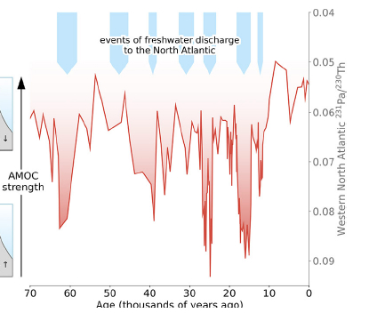
Figure II.14. Measurements of the 231Pa/230Th ratio in deep sea sediment samples from the Bermuda Rise region in the western North Atlantic, as a function of the inferred age of the sample. In the downward dips the ratio approaches the known production ratio for the two isotopes, indicating weak or missing AMOC transport of 231Pa. The most rightward downward spike corresponds to the Younger Dryas period and the melting of the Laurentide ice sheet during the deglaciation period following Earth’s last Ice Age.
The results in Fig. II.14 suggest many previous episodes of AMOC collapse or severe weakening. The most recent downward spike occurred roughly 12,000 years ago, during a well-known period called the Younger Dryas. During this period the massive Laurentide Ice Sheet, which covered a great deal of North America during the last Ice Age, was melting and depositing vast amounts of cold, fresh water in the North Atlantic, an event not unlike what might happen if the Greenland Ice Sheet undergoes massive melting as a result of global warming. Independent measurements of central Greenland temperatures from extracted ice cores show that the temperature dropped rather precipitously by about 10°C 12,900 years ago and recovered, again rather rapidly, only about 11,600 years ago. This episode in our planet’s climate prehistory offers insights into what might happen if our ongoing global warming leads to massive Greenland ice melt, a corresponding collapse of the AMOC, and a resulting North Atlantic (and Western Europe) deep freeze!
This section has thus highlighted some of the profound new insights that radiometric dating has provided in both archaeology and paleoclimate studies.
— Continued in Part II —
