Super El Niño Events are on the Rise

August 25, 2026

I. Introduction: Strong El Niño Global Impacts

The El Niño-Southern Oscillation (ENSO) cycle refers to an alternating pattern of prevailing wind and ocean currents over the Equatorial Pacific Ocean, with enormous impacts on weather patterns around the globe. Recent months have seen repeated warnings that during the current year (2026-7) the world is likely to experience the strongest El Niño event in at least the past 140 years and quite possibly much longer, with severe impacts on worldwide weather.

The warnings are based on quantitative measurements. A characteristic feature of ENSO is the surface and subsurface temperatures in the eastern-to-central Equatorial Pacific Ocean. Figure I.1 shows measured Pacific sea surface temperature anomalies in December 1997, in the midst of a very strong El Niño year, and December 1988, in the midst of a moderately strong La Niña year. The temperatures in each case are measured with reference to the average temperatures over a 30-year period from 1981 to 2010. The contrast between El Niño and La Niña is clear and stark.

There is a standard index – called the Oceanic Niño Index, or ONI — used to gauge the strength of El Niño and La Niña episodes, based on Pacific Ocean sea surface temperatures measured within the rectangle labeled Niño 3.4 in Fig. I.2, including latitudes from 5°N to 5°S and longitudes from 120°W to 170°W. When those temperatures exceed the 30-year average by more than +0.5°C, the conditions support an El Niño event; when they are more than 0.5°C below the 30-year average, the conditions support a La Niña episode. When the deviations exceed 2.0°C in magnitude conditions support a super episode of either type.

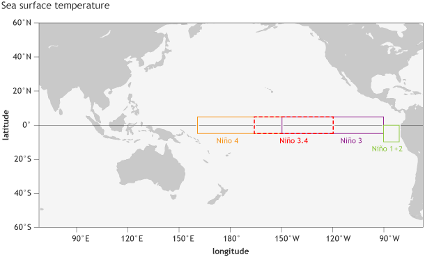
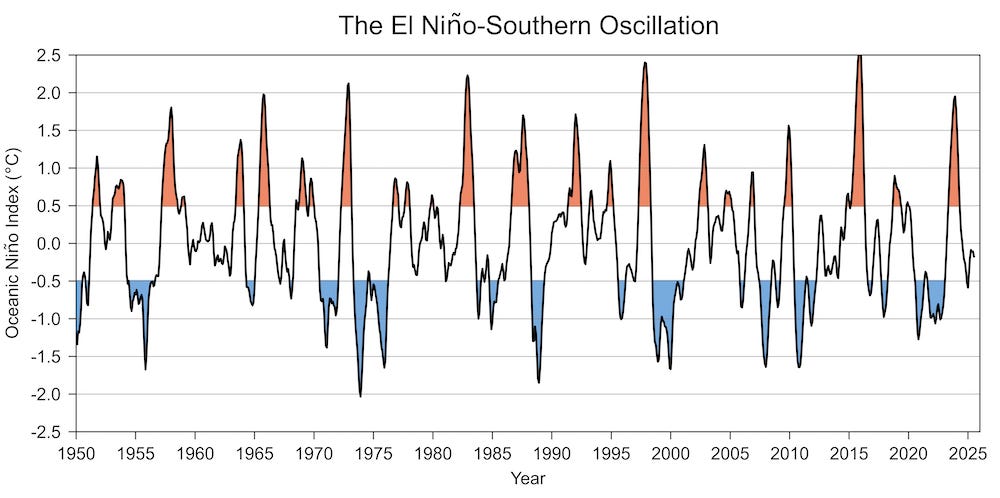
Figure I.3 charts the ONI as a function of time during the year, from 1950 to 2025. The red spikes correspond to El Niño years while the blue spikes correspond to La Niña. The white regions between +0.5°C and -0.5°C correspond to neutral conditions, which we will describe in more detail in Section II. One can see from the chart that we have already experienced super El Niño episodes (ONI above 2.0°C) in 1972-3, 1982-3, 1997-8, and 2015-16, and very nearly reached that level in 1965-6 and 2023-4. 2026-7 is predicted to be even more severe than the very strong episode in 2016.

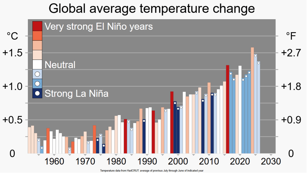
Strong El Niño events tend to amplify numerous impacts of ongoing climate change. Their impact on the global mean temperature anomaly is shown in Fig. I.4. The steady rise in global temperatures since 1970 is a feature of ongoing global warming, caused primarily by human emissions of greenhouse gases. But rising above the general trend, one can see local temperature peaks corresponding to strong El Niño episodes in 1972-3, 1997-8, 2015-16, and 2023-4.

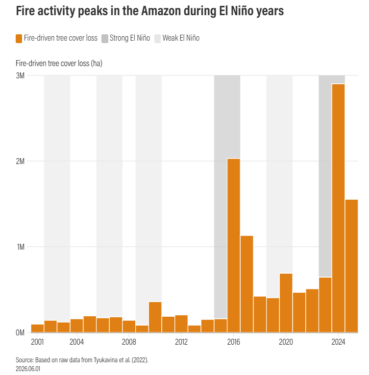
One of the impacts of strong El Niño episodes is to cause drought conditions in South America’s Amazon rain forest. Figure I.5 shows the fire-driven tree cover loss in the Amazon as a function of year during this century. Very strong peaks are seen in the strong El Niño seasons from 2015-16 and 2023-4. Another region susceptible to severe drought conditions during winter and spring of strong El Niño years is Southeast Asia. Figure I.6 shows forecasts for water availability in Southeast Asia during the super El Niño of 2015-16. Many locations there were forecast to suffer from severe water scarcity.

While strong El Niño episodes cause severe drought in some regions of the globe, they simultaneously greatly increase precipitation in other regions, such as Southern California in winter and early spring. The mechanisms for these variations around the world will be discussed in Section III. Figure I.7 shows that the average annual rainfall in Southern California is increased by about 60% on average in strong El Niño years.

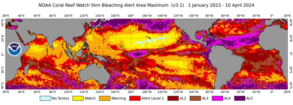
Strong El Niño years have also caused major global bleaching episodes for the world’s warm-water coral reefs. During the 1998 El Niño 21% of the world’s corals were bleached. In the subsequent strong El Niño years of 2010, 2016, and 2024, that bleaching percentage grew steadily to 37%, 68%, and 84%. Figure I.8 shows a National Oceanic and Atmospheric Administration (NOAA) map indicating the level of danger to global reefs during the 2024 episode, with colors from red to deep purple indicating progressively increasing alert levels. Reefs sometimes recover from bleaching episodes, if the ocean changes that cause the bleaching subside. But 30% of worldwide reefs have already been lost during the 21^st century and many more are at short-term risk from a super El Niño episode in 2026-7. Deaths of coral reefs severely impact ocean ecosystems. 25% of all marine species depend on reefs during some stage of their development. Furthermore, they support a great deal of fishing, providing not only food for humans but a livelihood for more than half a billion people. They also provide a buffer for coastal communities, helping to protect them from high waves, flooding, and storm surges.

In short, super El Niño episodes cause major disruption and worldwide weather disasters, with severe impacts on human health and economies. For example, the two strongest ones we have seen before this year, in 1997-8 and 2015-16 “brought catastrophic flooding to the eastern Pacific while plunging Africa, Australia and southeast Asia into severe droughts… The 1997-98 El Niño alone caused an estimated US$5.7 trillion (£4.4 trillion) in global income losses.” And as shown in Fig. I.9, current weather projections for 2026-7, based on the observed trend in Equatorial Pacific Ocean temperatures to date, are predicting a super El Niño that will be significantly stronger even than the one in 2015-16 (represented by the thin purple line in the figure). Furthermore, this year’s episode is occurring in a steadily warming world.

So, what might we expect in 2026-7? The World Resources Institute recently asked a number of experts to assess the world regions and systems that may feel the most severe impacts over the next year and a half. Here are some of their projections:

• “A Super El Niño would therefore destabilize the ocean systems that millions of people depend on for food, work, culture and protection from climate impacts.”
• “…areas expected to experience drought this year include the Caribbean, Central America, northern Brazil, central and northern India, central and southern Africa, Indonesia, the Philippines and Australia.”
• “…areas that may experience wetter conditions this year include the southern United States, parts of Peru, Ecuador, eastern Africa and parts of the Middle East and Central Asia.”
• “Regions already vulnerable to water stress may experience sharper declines in water availability. Flood-prone areas could see more damaging rain.”
• “Higher temperatures can make the atmosphere thirstier, pulling more moisture from soils and plants. This can dry out soils and crops faster, worsen heat stress for crops and livestock, and make droughts more damaging even when rainfall deficits are similar to past El Niños.”
• “The Iran-U.S. conflict-related fuel and fertilizer disruptions matter because they reduce resilience. A strong to very strong El Niño would raise the risk of drought, heat, flooding, pasture stress, fisheries disruption and regional crop losses in certain parts of the world. Those risks become more serious when farmers have fewer tools to respond.”
• “Potentially record-breaking forest fire activity in the Amazon is most likely in the second half of 2027, when reduced wet season rainfall leaves the following dry season even more arid and fire-prone. Elevated fire risk is also likely in Southeast Asia, Australia and Canada later this year and into 2027.”

Traditionally, it has been assumed that El Niño-La Niña cycles occur every two to seven years, but that super El Niños occur perhaps once every 15 years. It has been only ten years since the last super El Niño and the one in 2023-4 was nearly as strong. There is recent research that suggests that ongoing global warming is accelerating both the intensity and frequency of El Niño events, so that by mid-century roughly half of such events may reach severe levels. While El Niños tend to amplify climate change impacts, we will show in this post that human-caused climate change is also amplifying El Niño impacts. In order to do that, we will first discuss what neutral wind and ocean currents look like in the Pacific Ocean and around the globe (Section II). We will then explain how El Niño and La Niña alter these neutral patterns and disrupt global weather (Section III). Then, finally, we can discuss in Section IV why global warming can make these disruptions even more severe.

II. Weather Baselines: Trade Winds and Jet Streams

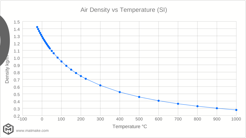
Earth’s baseline weather patterns, from which El Niño and La Niña cause alternating changes, is driven by surface and high-altitude winds that arise from air pressure differences around the Earth and the Coriolis effect from Earth’s continuous rotation about its axis. The density of air decreases as its temperature increases (see Fig. II.1). Thus, cold dense air tends to sink within the atmosphere, while hot air rises. Since Earth is heated unevenly by the Sun, temperature differences around the globe lead to air pressure differences. In particular, the warmest surface air at the Equator tends to rise, creating low surface air pressure along the Equator. Conversely, cold dense air at the poles sinks, creating a high-pressure region at both poles.

Air at Earth’s surface thus tends to flow from the high-pressure poles toward the low-pressure Equator. But the cold air flowing from the poles meets warmer air along the way and forces it upward. This creates another low-pressure region (the Polar low) about 60° in latitude in both the northern and southern hemispheres. The warm air rising from the Equator flows toward the poles at high altitude, while the less warm air rising from the Polar lows flows toward the Equator at high altitude. These two high-altitude air flows collide over the Earth at about 30° latitude in both hemispheres. The collision leads to a downward flow near 30°, creating a high-pressure region there – the subtropical highs — at the surface. These phenomena give rise to the wind patterns illustrated in Fig. II.2.

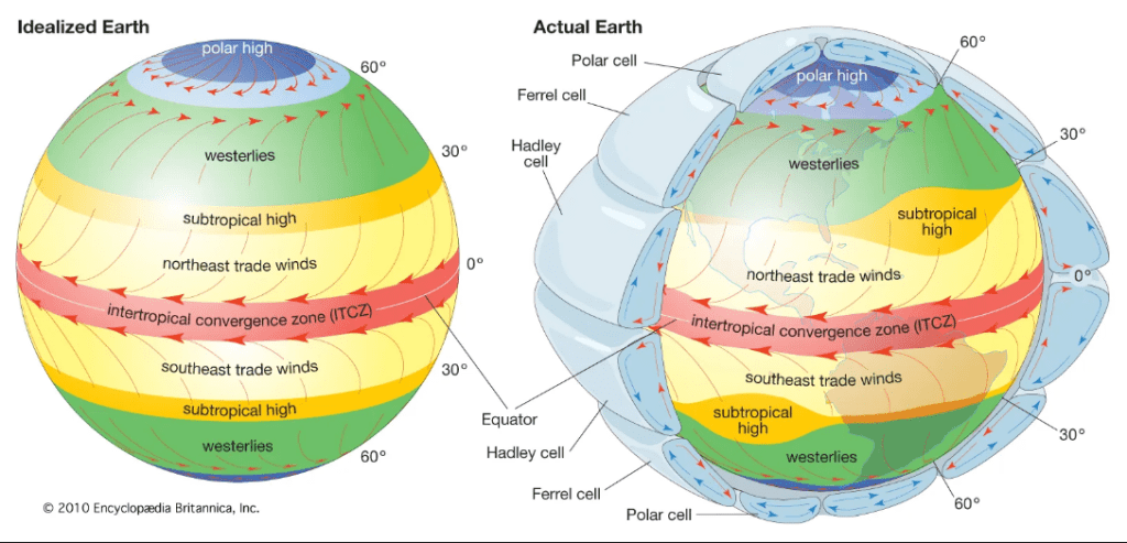
The left-hand globe in Fig. II.2 illustrates what high- and low-pressure regions and resulting surface wind patterns would look like if Earth’s surface were featureless. Surface winds tend to flow from the high-pressure regions at the poles and 30° N and S toward the low-pressure regions at the Equator and 60° N and S. These winds begin by moving in a north-south direction but then they get diverted by the Earth’s rotation. Earth’s atmosphere is dragged around with it, from west to east, as the Earth rotates about its axis. But the resulting eastward velocity of surface air is greatest at the Equator and decreases with increasing latitude. This occurs because all points on Earth complete one full rotation in one day, but the circumference of the circle that a point on the surface follows gets progressively smaller as one moves from the Equator toward the poles. Hence, when winds originating at 30°N or S reach the Equator, points on the Equator have moved eastward faster than that wind is moving eastward. To an observer on Earth, those winds then appear to have moved toward the west. The Equator-bound winds thus appear to have flowed from the northeast (30°N) or the southeast (30°S) and to be moving westward at the Equator. Where they meet, in the intertropical convergence zone, they produce prevailing winds flowing from the east toward the west. In a similar fashion, winds flowing poleward from the subtropical highs are moving faster toward the east than their destination points, so the winds appear as westerlies (i.e., originating in the west), flowing toward the east. These are the implications of the Coriolis effect.

The right-hand globe in Fig. II.2 takes into account Earth’s continental land masses and shows the vertical air flows as well. The subtropical highs now occur in the middles of the Atlantic and Pacific Oceans at 30°N and S. The vertical flows subdivide into three basic cells in each hemisphere. In the Hadley cells hot air rises from the Equator lows, cools at high altitude, and returns earthward at the subtropical high-pressure regions. Air rising from the polar lows at 60°N and S is returned to Earth either at the poles in the polar cell or at the subtropical highs in the so-called Ferrell cell.

At high altitude the air temperature changes rather abruptly across the boundaries between the Hadley and Ferrell cells and between the Ferrell and polar cells. As illustrated in Fig. II.3, these temperature changes give rise to narrow bands of high-velocity wind at high altitudes – the subtropical and polar jet streams. The air that feeds the jet streams originates in the rising hot air at the Equator, where that air has a much higher eastward velocity than at the latitudes of the cell boundaries; the air is thus moving eastward much faster than points on the Earth at 30° and 60° latitudes. The jet streams thus appear to observers on Earth to be moving from west toward the east around the Earth. The jet streams tend to occur from five to seven miles above the surface and at their centers the wind speeds can reach more than 200 miles per hour. They occur at altitudes comparable to those used in long-distance air travel and often have strong impacts on travel times and fuel consumption, speeding up flights heading east and slowing down flights heading west.

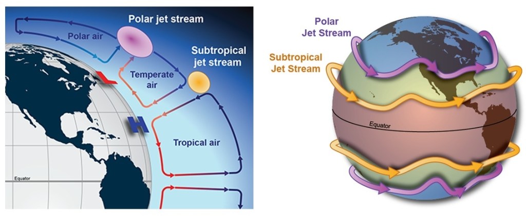
As illustrated in the right-hand image in Fig. II.3, the jet streams actually meander about the globe both in latitude and in altitude, following air pressure and temperature variations. Their precise location is also affected by the seasons. The jet streams tend to shift poleward in Spring, when the Sun’s elevation is increasing from day to day, and to shift toward the Equator in Autumn, when the Sun’s elevation is decreasing.

The trade winds and the jet streams have enormous influence over Earth weather. The surface winds drive major surface ocean currents called subtropical gyres, as illustrated in Fig. II.4. The warmest water at the Equator flows westward under the influence of westward trade winds in the Equatorial region. When the Equatorial ocean currents reach land boundaries – the eastern coasts of Asia, Indonesia, and Australia for the Pacific Ocean, the eastern coasts of North, Central, and South America for the Atlantic Ocean, and the eastern coast of Africa for the Indian Ocean – the currents turn away from the Equator in both northern and southern hemispheres. When those currents cross the subtropical high-pressure regions they become subjected to the prevailing westerly winds at the higher latitudes. These winds drive the now colder water back eastward to complete the gyres.

The density of seawater increases as its temperature cools toward the freezing point. Hence, under ordinary conditions cold, salty water tends to sink and warm, salty water remains at the surface. The warm water flowing away from the Equator in the gyres shown in Fig. II.4 thus tend to stay at the surface and to warm the eastern coasts bordering each ocean. They give these coasts mild and damp climates. In contrast, the warm near-Equator waters that are driven by the trade winds away from the eastern boundaries of the oceans allow deeper cold and nutrient-rich waters to well up to the surface in their place. These cold surface waters flow back toward the Equator to complete the subtropical gyres, giving the western coasts of North and South America, Africa, and Australia typically cool and dry climates. Furthermore, the upwelling cold water brings with it a great deal of marine life, providing a boon to fishing on the affected coasts.

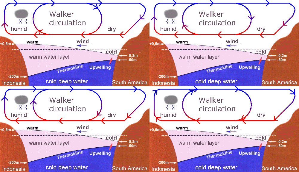
The combination of the trade winds and the subtropical gyres give rise to an east-west sea surface temperature and air pressure difference across the oceans in the tropics and to a resulting vertical air circulation pattern over the oceans, known as a Walker circulation cell. The Walker cell over the Pacific is illustrated under neutral conditions in Fig. II.5. The warmest water now in the western Pacific gives rise to rising hot air accompanied by evaporation and gives the western Pacific a lower atmospheric pressure than the eastern Pacific. The rising hot, moist air creates humid conditions, often with lots of rainfall, along the eastern coasts of Asia, Indonesia, and Australia. As that hot, moist air rises, it cools and dries and flows at altitude back toward the relatively higher-pressure region at the eastern reaches of the Pacific. There it falls, warms, and flows back to enhance the easterly surface trade winds to complete the Walker circulation.

The jet streams act like high-altitude conveyor belts, strongly influencing the development and movement of high-pressure and low-pressure weather systems, often steering storm systems around the globe. When the jet streams flow over regions where atmospheric pressure happens to be low, they tend to suck air up into the jet streams, causing further pressure drops and often stormier conditions. When the jet streams slow or buckle, they allow high-pressure weather systems to hang around, typically bringing calmer, drier weather and clear skies.

We will see in the next Section that El Niño and La Niña alter the Equatorial trade winds, the subtropical gyres, the Walker circulation, the locations of the jet streams, and hence, worldwide weather patterns.

III. El Niño and La Niña Impacts on Global Weather Patterns

The winds on Earth are, of course, variable around the baseline described in Section II. A typical El Niño episode begins with a weakening of the tropical trade winds that normally drive warmer Equatorial Pacific waters toward the eastern coasts of Asia, Indonesia, and Australia. That weakening is accompanied by wind bursts blowing from the western Pacific toward the eastern Pacific. These westerly wind bursts drive the warmer waters of the western Pacific back along the surface toward the east, enhancing the Ocean Niño Index (ONI), disrupting the Pacific subtropical gyres, and reversing the convective vertical air flows in the Walker circulation cell. Figure III.1 illustrates the changes from the Walker cell in both moderate and extreme El Niño years.

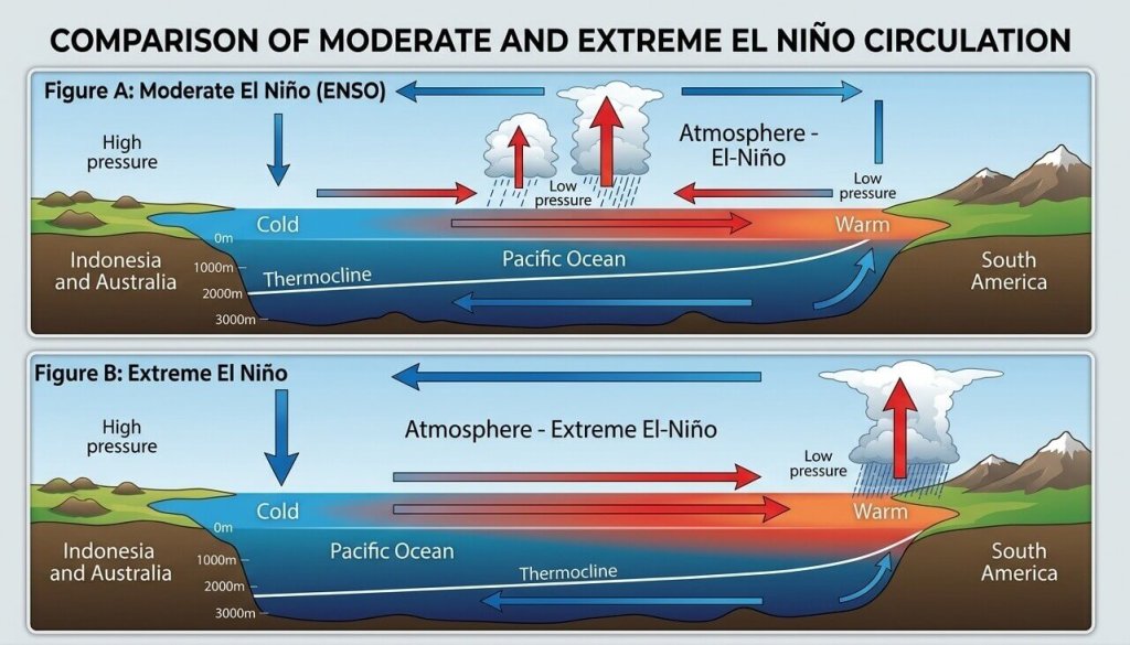
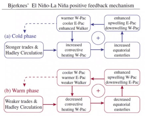
Recall from Fig. II.5 that under neutral conditions the Walker cell enhances the easterly surface trade winds across the Equatorial Pacific. When the trade winds weaken at the start of an El Niño, the Walker cell weakens as shown in the upper frame of Fig. III.1, further weakening the easterly surface winds and strengthening the westerly winds.  This drives warm water more forcefully toward the eastern Pacific, increasing the sea surface temperature (SST) gradient, further weakening the Walker cell and enhancing the westerly surface winds. This positive feedback loop, known as the  Bjerknes feedback, strengthens El Niño and eventually can lead to the extreme conditions shown in the lower frame of Fig. III.1, where the Walker cell is completely reversed. The elements of the Bjerknes feedback loop, which acts during both El Niño and La Niña events, are summarized in Fig. III.2.

Strong El Niño episodes not only reverse the Pacific Ocean Walker circulation but that reversal also changes vertical air flow patterns in tropical regions around the globe, as illustrated in Fig. III.3. All of those changes affect worldwide weather patterns.

La Niña episodes restore the east-to-west tropical trade winds but strengthen them. This makes the sea surface temperatures in the western Pacific even higher than the normal indicated in Fig. II.5 and the rising, hot, moist air flow at the eastern shores of Asia, Indonesia, and Australia, hence, the Walker circulation, even stronger than normal.

The ENSO wind pattern changes that occur over the Pacific Ocean cause wind pattern and atmospheric pressure changes around the globe. For example, Fig. III.4 compares high altitude atmospheric pressure changes from neutral conditions over the North Pacific coast and land mass of North America during El Niño vs. La Niña winters. The warm waters in the eastern Pacific during El Niño lead to an intense low-pressure region in the North Pacific off the western coasts of the U.S. and Canada, while the cooler eastern Pacific waters during La Niña lead to high atmospheric pressures in the same geographic region.

The stark pressure differences revealed in Fig. III.4 occur at altitudes characteristic of the jet streams. They therefore induce significant shifts in the location and extent of the Pacific jet streams during El Niño vs. La Niña years. As illustrated in Fig. III.5 the El Niño low-pressure system causes the subtropical north Pacific jet stream to move toward the south and to spread further east. The impact on North American winters is to produce wetter and cooler than normal conditions in the South and warmer and drier conditions in the North, below the Polar jet stream that marks the dividing point between temperate and polar climates. For example, “the very strong El Niño that began in 1997…saw weeks of drenching winter storms in California and heat records smashed in the Midwest and Northeast.”

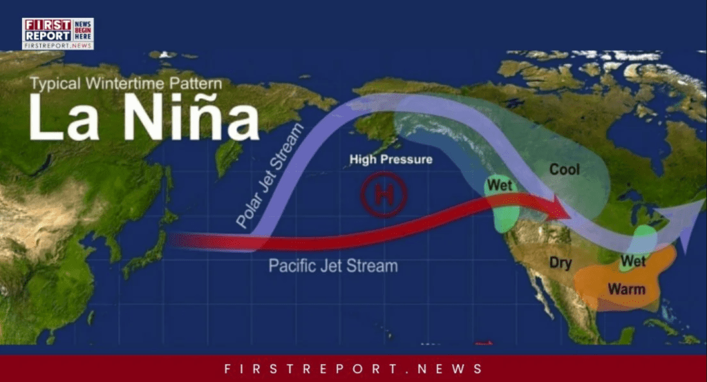
In contrast, as illustrated in Fig. III.6, La Niña conditions push the Pacific jet stream further to the north, so that it actually merges with the Polar jet stream over North America. This reverses the winter weather trend, producing wetter and cooler temperatures in the northern U.S. and Canada and warmer and drier conditions in the southern U.S. and parts of Mexico.

El Niño impacts on weather on other continents as a function of season are illustrated in Figs. III.7 and III.8. El Niño brings dry weather throughout the year to the northern and northeastern regions of South America, accounting for the extensive Amazon fire loss seen in Fig. I.5 in 2016 and 2024. At the same time, it brings wet weather and heavy rainfall to southern Brazil. Some examples of its effects: “severe floods in southern Brazil in 1982-83, drought in Colombia that ravaged coffee crops in 1997-98, and below-normal rain and wildfires in the Amazon in 2015-16.” Even though the 2023-4 El Niño was not quite as strong as its super predecessors, its effects in South America appear to have been enhanced by global warming: “The extra warmth increased evaporation, which supercharged drought in the Amazon. It also intensified the rains in Brazil’s south, because warmer air can hold more moisture.”

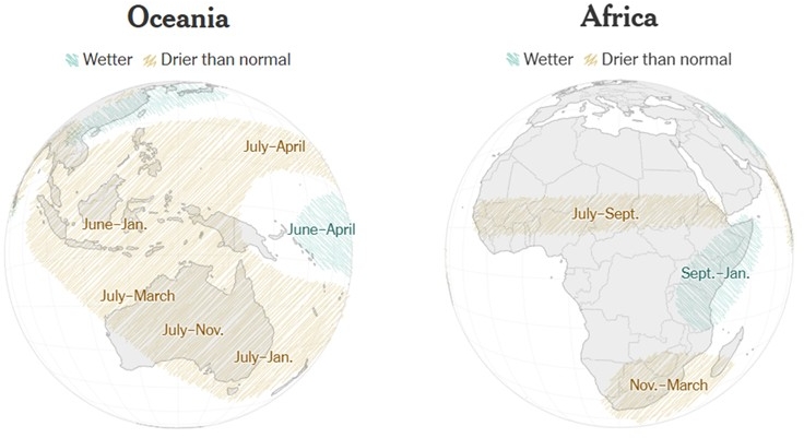
El Niño brings hot and dry weather to South and Southeast Asia, accounting for the water scarcity seen in Fig. I.6 for the 2015-16 super El Niño. At the same time, it brings wet weather and heavy rainfall in late Fall and Winter to eastern China. The super El Niño of 1997-8 caused China’s worst flooding in five decades, with some 3,000 people killed by Yangtze River overflow.

The dry conditions throughout Southeast Asia continue through Indonesia and Australia, as seen in Fig. III.8. In Africa El Niño tends to wipe out normal rainy seasons in the Sahel in summer months and in southern Africa in November through March. For example, “The 2015-16 El Niño caused crops to fail across southern Africa, with food production falling by two-thirds in some countries.” At the same time, it brings warm, moist air blowing in across the Indian Ocean (see Fig. III.3) toward East Africa, which often sees Fall and Winter “floods, landslides, and malaria outbreaks.”

All of these effects grow more severe during super El Niño years and many of the effects are getting further amplified by human-caused global warming.

IV. Global Warming is Making El Niño Events Stronger

There is no question that during El Niño years many of the negative impacts of human-caused global warming are made more severe. But we can also ask whether global warming is affecting the intensity, frequency, or extent of El Niño episodes. Are these effects, arising from supposedly independent drivers, mutually reinforcing?

Direct measurements of tropical Pacific Ocean temperatures only go back less than 150 years. During that period there have been at most a dozen recorded super El Niño episodes (see Fig. I.9), not enough to distinguish whether the frequency of such extreme events is changing over time. However, various researchers have considered proxies that provide some information on the strength of ENSO variability over thousands of years. For example, fossilized corals in the tropical Pacific Ocean can measure local temperatures via the ratio of various oxygen isotopes found within, and each fossil can be dated by ratios of radioactive nuclei and their decay daughters. These corals can provide a record going back at least 7,000 years. Similar analyses of the calcium carbonate shells of microscopic marine organisms known as foraminifera have provided measures of tropical Pacific Ocean ENSO variability going back to the Last Glacial Maximum (LGM) during the last Ice Age, 21,000 years ago. The same sort of oxygen isotope analysis has also been applied to stalagmites extracted from caverns in southeastern Alaska, which are sensitive to the North Pacific low atmospheric pressure region that accompanies El Niño events (see Fig. III.4) and provide records going back 3,500 years.

Such proxy measurements show clearly that the degree of variability from year to year in eastern and central equatorial Pacific Ocean temperatures was significantly smaller in the distant past than it is today. But in order to judge whether human-forced climate change is today increasing that variability and the frequency of extreme El Niño events, one must rely on global climate models that can handle the complex ocean-atmosphere coupling that leads to ENSO. Such models can be benchmarked by comparison to proxy data from past eras. Then the role of human forcing can be assessed by seeing how today’s variability compares to model calculations that turn off the human forcing. We discuss a few of these recent studies here.

Thirumalai, et al., have carried out simulations with “Community Earth System Model v.1.2… a model that realistically simulates key ENSO dynamics” during 3,000-year intervals going back to the LGM, thus spanning periods of glacial, interglacial, preindustrial, and human-forcing climate eras. They find the foraminifera proxy data for equatorial Pacific Ocean temperature variability during the Last Glacial Maximum to be in excellent agreement with their simulations.  The central results of their simulations are presented in Fig. IV.1. Frame (a) of the figure displays the simulated ENSO variability for nine different time periods, where the variability is defined as the standard deviation of simulated monthly sea surface temperature (SST) anomalies averaged over the Niño-3.4 region (see Fig. I.2) used to determine the Ocean Niño Index. The simulated variability decreases from the LGM until about 15,000 years ago, when huge ice sheets covering much of the Northern Hemisphere were melting, and then increases steadily to the modern era. The “present” era is represented by the purple box labeled PI for “preindustrial,” where human forcing has been turned off in the simulations. In order to represent the effect of human emissions of greenhouse gases, the authors also did a simulation for a future time (rightmost pink box) when atmospheric carbon dioxide concentrations reach a level twice that measured in the preindustrial era. At the present rate of human greenhouse gas emissions that condition is likely to be reached about 2060.

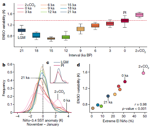
Frame (b) of Fig. IV.1 presents for each of the nine time periods the frequency distribution of simulated SST anomalies during November-to-January, the months when El Niño events typically peak. Inset (c) presents those same distributions for the LGM and PI periods only. Note that the LGM distribution is essentially Gaussian in shape, while the distributions for more recent periods develop first a shoulder and then a second peak at positive temperature anomalies. The secondary peak is especially prominent for the future period with atmospheric carbon dioxide concentration doubled from the preindustrial era. Super El Niño events increase in frequency as that secondary peak grows. In the doubled CO₂ simulation the primary distribution peak shifts toward negative values, which tends to also increase the frequency of strong La Niña events.

Frame (d) of Fig. IV.1 plots the correlation between the ENSO variability metric used in frame (a) and the fraction of El Niño events that reach super status (SST anomaly > 2.0°C). According to the simulations, fewer than 10% of El Niño events reached super status during colder, more distant eras. But that fraction had increased to about 1/3 in the preindustrial era and will increase further to ½ by about the middle of the 21^st century if humans continue emitting greenhouse gases at the current rate.

The Thirumalai, et al. simulations thus suggest that as the Pacific Ocean warms El Niño events grow stronger. By analyzing their simulations in detail the authors are able to suggest the mechanism by which this strengthening occurs. The model they propose, relying on changes in the strength of the Pacific Walker circulation and the Bjerknes feedback loop, is illustrated schematically in Fig. IV.2. Under cold global conditions, such as at the LGM, there is a strong SST gradient in the equatorial Pacific, with warmer water confined to the western Pacific. That gradient supports a strong Walker circulation that is resistant to reversal under El Niño conditions. At the same time the warm-cool mixed layer in the Ocean is deep, weakening the mechanical coupling by which westerly winds would be able to force warm surface waters further eastward. These factors combine to make the Bjerknes feedback loop weak, hence, to limit the occurrence of extreme El Niño events.

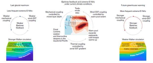
Under warm global conditions, as expected from continuing greenhouse warming, all of these effects are reversed. The equatorial warm waters naturally extend far toward the eastern Pacific, the SST gradient is weak under neutral conditions, and so is the Walker circulation. The Walker circulation is thus less resistant to reversal during El Niño. Furthermore, the mixed layer in the Ocean is now shallow and westerly winds have a stronger mechanical coupling to drive warm surface waters still further eastward. These are the conditions that lead to a strong Bjerknes feedback loop, which enhances the likelihood of extreme El Niño events.

Earth’s ocean-atmosphere coupling is complex but the mechanism of Fig. IV.2 certainly provides a plausible explanation for why super El Niño events may be on the rise as human emissions of greenhouse gases continue to warm the planet.

An independent set of climate simulations, now focusing primarily on the 20^th and 21^st centuries, has been carried out by Cai, et al. These authors used 39 independent global climate models tested in the sixth phase of the Coupled Model Intercomparison Project (CMIP6). They first turned off human forcing in the models to simulate the occurrence of El Niño events over a period of three centuries, in order to assess the degree of variability in the absence of human-caused global warming. With human forcing turned back on, they then simulated the occurrence of strong El Niño events within 60-year-long sliding windows, beginning in 1900, continuing to the present day, and projected out to 2100. Their simulation results for the frequency of both strong El Niño and La Niña events are shown in Fig. IV.3.

Even allowing for the spread and fluctuations of baseline results from preindustrial conditions and for the additional spread of results from different models including human forcing, the Cai results suggest that human-caused global warming is increasing the frequency of extreme ENSO events. The mean results suggest that since about 1960, as global warming has steadily raised temperatures around the planet, the frequency of strong El Niño events has increased from a baseline of four per century to a present value of more than six per century, and will increase further with continued global warming to more than eight per century by 2100.

Note that the results in Fig. IV.3 represent absolute frequencies, while those in Fig. IV.1(d) represent relative frequencies. A future later this century in which one of every two El Niño events is extreme, as suggested in Fig. IV.1, is not inconsistent with one in which such extreme events occur roughly once every 12 years. In addition, the Cai simulation result suggesting that the present return period for super El Niño is about 15 years is not inconsistent with our experiencing three such events from 1997-8 to 2026-7.

Other recent analyses have suggested an impact of global warming also on the duration of ENSO periods. Lu, et al. combined an analysis of Pacific Ocean fossil corals with multiple global climate models to show that “the ratio of multi-year to single-year ENSO events increased by a factor of 5” over the past 7,000 years. Geng, et al. use global climate models to project a future significant increase in the frequency of consecutive La Niña events under the influence of continuing human greenhouse emissions. The latter authors point out that “Multi-year La Niña events tend to follow a strong El Niño. For example, all three extreme El Niño events in the twentieth century (1972/73, 1982/83 and 1997/1998) were followed by multi-year La Niña events… The multi-year La Niña events occur because a large upper-ocean heat discharge of the equatorial Pacific induced by the strong El Niño requires more than one La Niña event to recharge to the climatological state, as the recharge process during La Niña is generally weaker than the discharge associated with El Niño.”

The climate models in all of these studies are consistent with the mechanism described in Fig. IV.2 as the cause of increasingly severe El Niño events as the globe continues to warm. As super El Niño events become more frequent, the impacts of climate change will grow more severe.

V. Conclusions

El Niño reverses sea surface temperature gradients across the equatorial Pacific Ocean, as well as prevailing winds, convective air flows, surface ocean currents, and atmospheric pressure variations around the Pacific region. Those reversals cause latitudinal shifts to the high-altitude jet streams that affect much of Earth’s weather. The net results are dramatic changes in temperature and precipitation patterns in all regions of the globe, occasionally leading to extreme flooding, drought, wildfires, storms, and heat waves in various regions.

El Niño events are strengthened by a positive Bjerknes feedback loop that arises from the thermodynamic and mechanical coupling between Pacific Ocean currents and winds. The vast majority of heat returned to Earth by greenhouse gas molecules in the atmosphere resides in the oceans. As humans continue to emit large quantities of greenhouse gases, the heat stored in the oceans will continue to increase. And global climate models suggest that as the Pacific Ocean continues to warm, the Bjerknes feedback will strengthen, and so will El Niño. We are currently heading into possibly the strongest El Niño event ever experienced by humans in 2026-7.

We have written previously about the nonlinearity of future climate change as one or more Earth systems pass climate tipping points. The mutual reinforcement between super El Niño events and human-caused global warming provides another mechanism contributing to such nonlinearity. Super El Niño events amplify climate change impacts, while human emissions of greenhouse gases appear to be increasing the frequency of super El Niño events. As a result of this reinforcement, we can expect more frequent and more severe extreme weather events over the coming decades.

Ignoring the fact of global warming and rejecting efforts to mitigate its impacts is a deeply foolish policy. Unfortunately, it is the policy of the present U.S. federal government. And it promises to bring all of the Earth’s inhabitants even more misery from extreme weather events throughout the 21^st century.

References:

National Ocean Service, What are El Niño and La Niña?,  https://oceanservice.noaa.gov/facts/ninonina.html

G. Patrick, What Makes This Year’s Super El Niño the Strongest in 140 Years? Causes Explained, The Science Times, May 2, 2026, https://www.sciencetimes.com/articles/61757/20260502/what-makes-this-years-super-el-nino-strongest-140-years-causes-explained.htm

A. Flis, Atmospheric Code Red: 2026 Super El Niño Now Trending Toward Record-Breaking Intensity, Severe Weather Europe, June 11, 2026, https://www.severe-weather.eu/long-range-2/super-el-nino-2026-record-breaking-intensity-forecast-weather-impacts-united-states-canada-europe-fa/

R. Lindsey, Climate Variability: Oceanic Niño Index, Climate.gov, Aug. 30, 2009, https://www.climate.gov/news-features/understanding-climate/climate-variability-oceanic-nino-index

A. Hoell, The El Niño-Southern Oscillation and Drought Outlook in the United States, NOAA Physical Sciences Laboratory, Sept. 8, 2025, https://econcurrents.substack.com/p/an-informative-article-on-enso-from

S. Parsons, How Might a ‘Super El Niño’ Affect Food, Forests and Water?, World Resources Institute, July 7, 2026, https://www.wri.org/insights/super-el-nino-impacts-explained

Wikimedia Commons, Global Surface Temperature Bar Chart – Bars Color-coded by El Niño and La Niña Intensity, https://commons.wikimedia.org/wiki/File:20210827_Global_surface_temperature_bar_chart_-_bars_color-coded_by_El_Ni%C3%B1o_and_La_Ni%C3%B1a_intensity.svg 

iSciences, Southeast Asia & the Pacific: Water Deficits to Persist in Southeast Asia, Borneo, New Guinea, Nov. 23, 2015, https://www.isciences.com/blog/2015/11/17/southeast-asia-the-pacific-water-deficits-to-persist-in-southeast-asia-borneo-new-guinea

My NASA Data, El Niño Southern Oscillation, May 18, 2015, https://mynasadata.larc.nasa.gov/basic-page/el-nino-southern-oscillation

Percentage of Reefs Bleached in Global Coral Bleaching Events, https://reefscapers.com/climate-charts/

Coral Reef Watch, Current Global Bleaching: Status Update & Data Submission, June 2, 2026 https://www.coralreefwatch.noaa.gov/satellite/research/coral_bleaching_report.php

Z. Lu, Consecutive El Niños are Happening More Often and the Result is More Devastating – New Research, The Conversation, Apr. 3, 2025, https://theconversation.com/consecutive-el-ninos-are-happening-more-often-and-the-result-is-more-devastating-new-research-251504

K. Thirumalai, et al., Future Increase in Extreme El Niño Supported by Past Glacial Changes, Nature 634, 374 (2024), https://www.nature.com/articles/s41586-024-07984-y

National Oceanic and Atmospheric Administration, The Jet Stream,  https://www.noaa.gov/jetstream/global/jet-stream

Weatherstem, How Do Gyres Affect Climate?, https://learn.weatherstem.com/courses/wxstem_meteorology_01/module-06/03/07.html

T. Di Liberto, The Walker Circulation: ENSO’s Atmospheric Buddy, https://www.weather.gov/media/wrn/walker-circulation.pdf 

PMF IAS, El Niño, https://www.pmfias.com/el-nino-el-nino-southern-oscillation-enso-indian-ocean-dipole-iod-la-nina-el-nino-modoki/

Met Office, What is the Jet Stream and How Does it Affect Our Weather?, May 28, 2025, https://www.metoffice.gov.uk/blog/2025/what-is-the-jet-stream-and-how-does-it-affect-our-weather

Bohrium, Bjerknes Feedback, https://www.bohrium.com/en/sciencepedia/feynman/keyword/bjerknes_feedback

Murtugudde Climate Academy, Bjerknes Feedback and ENSO Theories https://www.youtube.com/watch?v=tKv4l7knoiA  

E. Becker, What We Talk About When We Talk About the Jet Stream and El Niño, Climate.gov, Sept. 29, 2023, https://www.climate.gov/news-features/blogs/what-we-talk-about-when-we-talk-about-jet-stream-and-el-nino

R. Zhong and H. Stevens, A Strong El Niño May Be Coming. Global Warming is Changing Its Effects, New York Times, May 4, 2026, https://www.nytimes.com/2026/05/04/climate/el-nino-global-warming.html

Weather.gov, Potential Impacts of Record-Breaking El Niño for North and Central Georgia, https://www.weather.gov/ffc/elninoimpactsnorthandcentralga

C. Davis, La Niña, Other Atmospheric Patterns Set to Shape Our Winter Weather, North Carolina State Climate Office, Nov. 15, 2016, https://climate.ncsu.edu/blog/2016/11/la-nina-other-atmospheric-patterns-set-to-shape-our-winter-weather/

B. Clarke, et al., Climate Change and El Niño Behind Extreme Precipitation Leading to Major Floods in Southern Brazil in 2024, npj Natural Hazards 3, article #4 (2026), https://www.nature.com/articles/s44304-025-00162-8

K.M. Cobb, et al., Highly Variable El Niño-Southern Oscillation Throughout the Holocene, Science 339, 67 (2013), https://www.science.org/doi/10.1126/science.1228246

P.S. Wilcox, M. Mudelsee, C. Spötl, and R.L. Edwards, Solar Forcing of ENSO on Century Timescales, Geophysical Research Letters 50, e2023GL105201(2023),https://agupubs.onlinelibrary.wiley.com/doi/10.1029/2023GL105201  

W. Cai, et al., Anthropogenic Impacts on Twentieth-Century ENSO Variability Changes, Nature Reviews Earth & Environment 4, 407 (2023), https://www.nature.com/articles/s43017-023-00427-8

CMIP6 – Couples Model Intercomparison Project Phase 6, https://pcmdi.llnl.gov/CMIP6/

Z. Lu, et al., Increased Frequency of Multi-Year El Niño-Southern Oscillation Events Across the Holocene, Nature Geoscience 18, 337 (2025), https://www.nature.com/articles/s41561-025-01670-y

T. Geng, et al., Increased Occurrences of Consecutive La Niña Events Under Global Warming, Nature 619, 774 (2023), https://www.nature.com/articles/s41586-023-06236-9

DebunkingDenial, Climate Tipping Points: Coming Soon to a Planet Near You?, https://debunkingdenial.com/climate-tipping-points-coming-soon-to-a-planet-near-you/