
April 18, 2024
I. Introduction
Global climate change has placed great stress on our environment. We are already seeing major effects from climate change. The oceans are retaining heat much faster than the rest of the globe, leading to rapid melting of sea ice and permafrost. Catastrophes such as hurricanes and wildfires are growing in severity, as a result of global warming. Significant portions of our food supply, such as seafood and crops, are under stress. However, climate change is now providing new threats to our ecosystem, in the form of “tipping points.” A tipping point represents a state of a system beyond which the system makes an abrupt transition to a new equilibrium point.
This is shown schematically in Figure I.1, which shows a ball in a valley in one dimension. The left-hand picture shows a ball in a state of stable equilibrium. The ball initially rests in a valley. Small excursions away from the equilibrium point require energy input and produce a “restoring force” that returns to ball to its equilibrium point. The middle curve shows a potentially unstable state. If the ball moves to the left, it will experience a restoring force that will send it back to its equilibrium point. For sufficiently small excursions to the right, the ball will also return to its equilibrium point. However, if the ball moves past the “hill” on the right-hand side, it will experience forces that move it down into the lower-energy valley at the right. The top of the hill on the right (denoted by the arrow) represents the ”tipping point” – if the ball moves past the tipping point, it will roll down into the new equilibrium point at the right.

Figure I.1: Schematic picture of tipping points. Left: a ball in a valley; the ball is stable to small deviations from its equilibrium point. Middle: if the ball moves sufficiently far to the right of its equilibrium point, it can “tip” and transition to a new equilibrium point. Right: the ball has moved from its original position to a new equilibrium point.
For an environmental system, a tipping point represents a state beyond which the system can move abruptly to a new equilibrium state. Once a system passes a tipping point, it may initiate adverse changes that are difficult or even impossible to reverse on time scales comparable to human lifetimes. If systems pass a tipping point, the results could be catastrophic. One example is warm-water coral reefs. These systems are host to a greater density of species per unit area than any other ocean area. Nearly half of all fisheries in the U.S. obtain their living from coral reef systems. Also, coral reefs provide significant support from tourists. Including fishing and tourism, it is estimated that global reef systems provide a source of income for over 500 million people. If coral reefs were to die off on a global scale, this could result in lower catches of seafood and dramatic decreases in tourism. This would have significant negative outcomes for people living in reef areas. Furthermore, it would disrupt ocean ecosystems.
Another area that could experience a tipping point is the North Atlantic sea circulation system. If sufficient melting of the Greenland Ice Sheet (GrIS) occurs, it could inject massive amounts of freshwater into the ocean. This might slow or even shut down the Gulf Stream, a body of warm water that moderates temperatures in Western Europe. If the Gulf Stream slows or shuts down, temperatures in Western Europe could plummet, even as the rest of the globe continues to warm; this could threaten European agriculture. It would also subject European populations to much lower temperatures; some models suggest that average temperatures in a country like Finland could decrease by 20o C.
If climate tipping points are reached, they could cause “cascading stress” to societies and economies. That is, passing a tipping point for one system may push other areas past another tipping point. An example of this is melting of the Greenland Ice Sheet; as we just mentioned, if the GrIS melts sufficiently rapidly, it could push the North Atlantic seawater circulatory system past its own tipping point. The Global Tipping Points report states that the impacts of climate tipping points could threaten the breakdown of economic, social and political systems. The impact of such changes will be profoundly unequal. Societies that have limited resources will be most likely to feel the devastating impact of such changes. The global governance system stepped up admirably in dealing with the ozone layer emergency. Every nation joined in a consortium to ban the use of chlorofluorocarbons, and under the Montreal Protocol they provided money and technical assistance to Third World countries (this is detailed in our blog post about the ozone controversy). It remains to be seen whether any comparable international collaboration can be mounted to deal robustly with the vastly more complicated and more expensive climate change issues.
One of the only ways to provide quantitative estimates regarding tipping points is to use models for the dynamics of these systems. The models are useful in that one can change various inputs to the system and predict the outcome. These climate models are thus able to probe how the system would respond to changes in input conditions, e.g. in the magnitude of the increase in global temperatures. However, these climate models are attempting to simulate exceptionally difficult situations, namely the interaction of one highly non-linear dynamical system (the atmosphere) with a second such system (the oceans). As a consequence, predictions of the global temperature increase at which various tipping points will be reached have large uncertainties. Nonetheless, we should maintain a healthy skepticism regarding the predictive powers of these models. However, because the consequences are so dire, we need to take the identification of systems susceptible to tipping very seriously. In some cases, we are helped because these climate systems may have passed tipping points in earlier eras. Thus, we can sometimes make use of paleo-climate data to test our climate models.
It is frightening to consider that various global systems could reach “tipping points” in the near future. This area needs considerably more study and governments need to redouble their efforts to minimize the effects of fossil fuel emissions and other drivers of climate change.
II. Tipping Points for Five Climate Systems
In 2023 a group at the University of Exeter issued a Global Tipping Points Report. This exhaustive 500-page report provides extraordinary details regarding the status of major climate systems and the potential that various systems could reach tipping points in the future. The Exeter report listed the five major climate systems that are in the greatest danger of reaching tipping points at the current level of global warming. These climate systems are:
- Warm-water coral reefs
- The Greenland Ice Sheet
- The West Antarctic Ice Sheet
- The North Atlantic Subpolar Gyre Circulation System
- Permafrost
In this post, we will review the five systems targeted by the Exeter Global Tippings Report as being closest to reaching tipping points at present. For each of these systems we will review their current status. Warm-water coral reefs are discussed in Section II.A. In Section II.B we discuss both the Greenland ice sheet and the West Antarctic ice sheet. We review the situation with the North Atlantic Subpolar Gyre and the coupled Atlantic Meridional Overturning Circulation systems in Section II.C. And we discuss potential tipping points for permafrost in Section II.D. We will discuss climate models and share their predictions for the fate of these systems. And we will discuss the uncertainties that accompany these predictions. The Exeter Group urges that a number of steps be taken to address the possibility of tipping points. First, they call upon the Intergovernmental Panel on Climate Change (IPCC) to include discussions of tipping points in its reports. Second, they suggest convening an international conference to address these issues. They also urge that climate studies address several of the outstanding questions regarding potential tipping points.
II.A: Warm-Water Coral Reef Tipping Points:
Coral reefs are among the most ecologically diverse and valuable ecosystems on Earth. On coral reefs, one finds “more species per unit area than any other marine environment, including about 4,000 species of fish, 800 species of hard corals and hundreds of other species.” However, coral reef systems are likely even more diverse than we realize. “Scientists estimate that there may be millions of undiscovered species of organisms living in and around reefs.” Coral reef systems support a great deal of fishing, for roughly half the U.S. managed fisheries. “The National Marine Fisheries Service estimates the commercial value of U.S. fisheries from coral reefs is over $100 million.” Worldwide, it is estimated that reef systems provide livelihood for over half a billion people. When healthy, as shown in Figure II.A.1, coral reefs supply resources to a vast array of living organisms. It is estimated that 25% of all marine species have life stages that are dependent on coral reef systems. Many of the organisms that thrive in reef systems are found nowhere else on Earth. In addition, warm-water coral reefs provide ample income through an array of tourism activities.
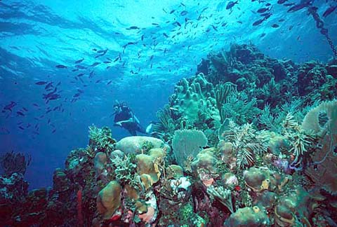
Figure II.A.1: A healthy coral reef system supports an incredibly diverse collection of marine life.
Figure II.A.2 shows the distribution of warm-water coral reef systems around the globe. With the exception of Europe, every continent has extensive systems of coral reefs.
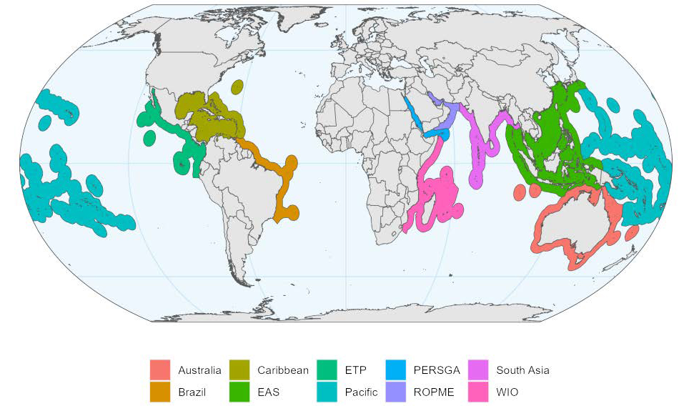
Figure II.A.2: Distribution of warm-water coral reef systems around the globe.
Coral reef environments also provide a buffer to coastal communities. They protect these communities against the energy that would otherwise buffet the coasts from high waves, flooding and storms. However, warm-water coral reef systems are also fragile. In particular, they are threatened by several different aspects of climate change. Figure II.A.3, from the National Oceanic and Atmospheric Administration (NOAA), highlights several ways that climate change is threatening coral reef ecosystems.
- Warming oceans produce thermal stress that causes bleaching;
- Sea level rise produces increased sedimentation that can smother coral;
- Stronger and more frequent storms can destroy reef structure;
- Increased runoff of sediment and pollutants can produce algal blooms and reduce the sunlight that reaches the corals;
- Altered ocean currents can diminish the food for corals and hamper dispersal of coral larvae;
- Increased ocean acidification can affect the integrity of the reef and decrease the rate of growth of the reef.
In addition to the threats to coral reef systems listed in Fig. II.A.3, other threats to warm-water coral reef systems include overfishing, disruption from passing ship traffic, and introduction of invasive species.
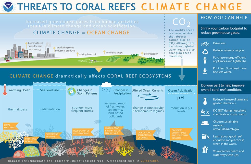
Figure II.A.3: Global Climate Changes That Can Harm Coral Reef Ecosystems. The figure from NOAA shows that various aspects of climate change are threatening coral reef systems. These include warming oceans that subject corals to thermal stress; sea level rise that produces more sedimentation; stronger and more frequent storms that can threaten coral reef structures; altered ocean currents that can diminish the food required by corals; and ocean acidification that can decrease coral growth.
Since the coral reefs under consideration require warm ocean conditions, it may seem paradoxical that increased ocean warming is threatening these ecosystems. The most common reaction of coral systems to various types of stress is a phenomenon called bleaching. As shown schematically in Fig. II.A.4, under normal conditions corals play host to algae called zooxanthellae. The algae live in the tissues of the coral, form the main food source for the corals, and provide the corals with their color. Both the corals and the algae benefit from this symbiotic relationship. However, when corals are stressed by the factors summarized in Fig. II.A.3, the algae can be expelled from the corals. When this occurs, the corals lose their color and turn bone white; this is the phenomenon called bleaching.
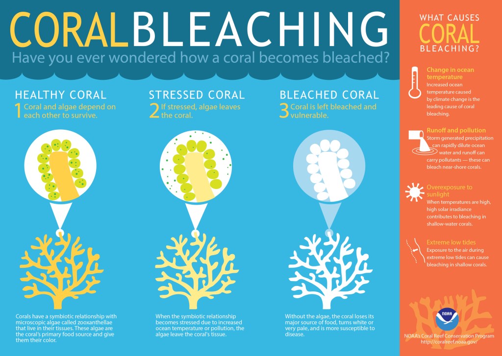
Figure II.A.4: Coral Bleaching. Under normal circumstances, algae live in the tissues of coral, in a symbiotic relationship. However, if stressed, the algae are expelled from the coral; the coral then turns white and becomes vulnerable to further, possibly permanent, damage. This phenomenon is known as coral bleaching.
Bleaching does not necessarily kill the corals, but it leaves them more vulnerable to further damage. There are cases where bleaching events are reversible; when temporary conditions that caused the bleaching abate, algae can return to the corals and they can regain their health. Another feature of the stresses listed in Fig. II.A.3 is that they make it more difficult for corals to build their skeletal structures. However, if the stressful conditions persist or if further stress is placed on the reefs, this can permanently kill the coral. The Great Barrier Reef Foundation states that climate change is the biggest threat to the future of coral reefs around the world. In just seven years, heatwaves have triggered four mass coral bleaching events on the Great Barrier Reef, and the effects of climate change have already reduced shallow water coral reefs by as much as 50%. Between 2004 and 2018, ten cyclones of category three or greater crossed the Great Barrier Reef, causing significant damage.
In the US, half of the coral reefs in the Caribbean were lost to a massive bleaching event in 2005. The thermal stress from this event was measured to be greater than that experienced in this region over the previous 20 years combined. A recent study of global reef structures during the period 1997 – 2018 found that “particularly marked declines in coral cover occurred in the Western Atlantic and Central Pacific.” Prof. David Baker of the University of Hong Kong stated that “The frequency and severity of mass coral bleaching events is increasing and indisputable. Corals have adapted to change over geological timescales – however, their evolutionary history has never encountered the unprecedented rate of change we are seeing.”
The various threats to coral reef systems can take place over different time periods. Thermal stresses, in particular, can occur over periods of weeks to months. On the other hand, threats such as disease to the corals, or from sedimentation that arises from runoff from farms, or sewage from onshore developments, can occur over periods of years. It is also the case that several of the threats listed in Fig. II.A.3 can act synergistically, so that the net effect on coral systems is larger than the individual factors. In general, a coral reef system is deemed to be ‘collapsed’ if the reef fails to recover over a period of a decade or longer.
Thermal stress is the primary driver of mortality to hard corals (see here and here); increasing ocean temperatures due to climate change are exacerbated by even more extreme conditions that occur during El Niño episodes. Figure II.A.5 shows a coral reef bleaching event that occurred in American Samoa in 2015. The panels of the figure show a healthy reef before the event (left), an area of the reef while it was experiencing the bleaching event (center), and dead areas of the reef following the bleaching (right). Figure II.A.6 shows coral bleaching episodes that have occurred around the globe over a 20-year interval (1998 to 2017). The figure is color-coded, where white indicates no bleaching; blue indicates average bleaching of 1% of the total area; and yellow indicates bleaching of 100% of the reef. As can be seen, damage to coral reef systems is occurring across the globe.
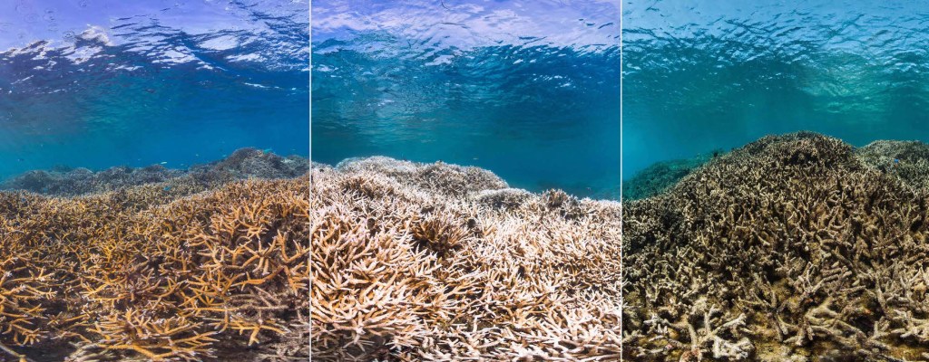
Figure II.A.5: A coral reef in American Samoa that experienced a bleaching event in 2015. Left: reef prior to bleaching event; center: reef during bleaching event; right: following the bleaching event, showing areas of dead coral.

Figure II.A.6: Coral reef bleaching events, episodes that have occurred around the globe over the interval 1998 — 2017. The figure is color-coded: white indicates no bleaching; dark blue indicates average bleaching of 1% of the total area, and yellow indicates bleaching of 100% of the reef.
The Sixth Assessment Report in 2022 (AR6) from the Intergovernmental Panel on Climate Change (IPCC) assigned “high confidence” to the statement that warm-water coral reef systems are suffering increased bleaching and mortality, and that these impacts have been attributed to human-induced climate change. In the future, IPCC report AR6 predicts that the climate change currently projected to occur, combined with ‘non-climatic drivers,’ is expected to cause loss and degradation of much of the world’s coral reefs with ‘very high confidence.’ And near-term risks for biodiversity loss are high to very high in warm-water coral reefs systems, with ‘very high confidence.’
So, warm-water coral reefs around the world are already experiencing significant mortality from a variety of effects due to global climate change caused primarily by human activity. For our purposes, global or regional “tipping points” for coral reefs would constitute reef mortality over much wider areas than we see at the moment; current reef damage tends to occur in regions of approximately 1,000 kilometers in extent. A tipping point would develop when relatively local damage expanded to regional mortality; under the most extreme conditions, reef damage might occur across the globe. Although conditions vary considerably across regions, we are already seeing extended reef damage. Over the past 50 – 150 years, the 2023 Global Tipping Points report estimates that about 50% of global coral reefs have been lost. It is estimated that in 1998 alone, 16% of global coral reefs were lost, and another 14% of reefs were lost during the period 2009 – 2018.
Models of reef systems attempt to take into account how the reefs will react to stresses placed on them. The most important single variable here is the average global temperature increase over the average global temperature from pre-industrial times. Cooley et al. estimate that global warming of 1.5o C will result in the loss of 70 – 90% of coral reefs; at warming of 2o C, this would increase to 99%. Currently, we have reached global warming of 1.2°C. During the period 1986 – 2019, “84% of global reef systems were estimated to experience ‘good’ thermal regimes.” Dixon et al. estimate that if global mean temperatures increase by 1.5o C by 2100, reefs with good thermal regimes would decrease to 0.2%, and an increase of 2o C would mean that no reef systems would have good thermal regimes.
What is the Evidence for Coral Reef Tipping Dynamics?
There are two possibilities for the threats to warm-water coral reefs. The first is that reefs are adapting to local conditions, so that the damage to reefs is simply a result of local effects. The second possibility is that large-scale regional or global ‘tipping points’ may be approaching. The Exeter Global Tipping Point report lists some evidence that global effects on reefs may be occurring.
- The first global coral reef bleaching event occurred in 1998; at this time global temperature increase was approximately 0.6o C, accompanied by a strong El Niño. Since that time, coral bleaching and mortality has occurred over larger regions and has increased in frequency and intensity.
- The Sixth IPCC Assessment report predicts that most warm-water reef systems will experience large-scale damage and degradation with “very high confidence.”
- Cooley et al. predict that the majority of coral reef systems around the globe are already passing tipping points for thermal bleaching.
- All coral reef systems are predicted to be at high risk for collapse. The status of the MesoAmerican Barrier Reef is Endangered, Western Indian Ocean coral reefs are Vulnerable, and Obura estimates that two-thirds of other reef systems are Endangered or Critically Endangered because of projected warming.
On April 15, 2024, the NOAA announced that exceptionally high ocean temperatures will cause the largest global bleaching event ever recorded this year. The economic value of the world’s coral reefs has been estimated at $2.7 trillion annually. This will be the fourth global coral bleaching event and is expected to affect more reefs than any other. Models from NOAA and its partner the International Coral Reef Initiative are used to predict damage to reefs. To qualify as a global bleaching event, all three ocean regions that host coral reefs – the Pacific, Indian and Atlantic – will experience bleaching within one year, and at least 12% of reefs in each basin must be subjected to high temperatures that cause coral bleaching.
The three previous global bleaching events have been increasingly severe; while the 1998 event affected 20% of the world’s reef areas, the 2010 event affected 35%, and the 2017 event affected 56% of coral reefs. The only good news is that the current El Niño that is heating the oceans is weakening; it is expected to give rise to a La Niña event that will cool the oceans somewhat. It is possible that this will allow reefs to heal and reverse the bleaching. However, overall the situation for warm-water coral reefs is bleak, as global temperatures continue to rise. We emphasize that models of reefs are simplistic and should be approached with some skepticism; however, current damage to reef systems is well documented, so we should take these model estimates quite seriously.
We should note here that the definition of a “tipping point” is somewhat different for coral reefs than for the other systems studied in this post, namely ice sheets, North Atlantic circulating currents, and permafrost. In those cases, the “tipping point” looks like the situation shown below in Fig. II.C.4; a situation arises where a small change in some variables results in “tipping” to a new state as shown schematically in Fig. I.1. For coral reefs, as global temperatures increase, all of the conditions in Fig. II.A.3 become more severe. Thus, model simulations estimate the amount of damage to coral reefs at a given temperature increase. As the temperature Increases, coral reef bleaching occurs over larger and larger areas, and more often results in reef collapse. When the extent and severity of the reef damage reaches a certain point, this is defined as a global “tipping point” for warm-water coral reefs.
Figure II.A.7 summarizes climate tipping points that have been reached or are predicted to be reached in ocean systems across the globe (from Cooley et al.). They are divided into three general categories. The first of these is losses in ice cover; the second is damage to coral reef systems; and the third is damage to large-scale kelp forests. For each region and tipping point, the impacts are divided into three general categories. The first is climate change hazards, the second category shows the social impact on various groups, and the third category is economic implications of these changes.
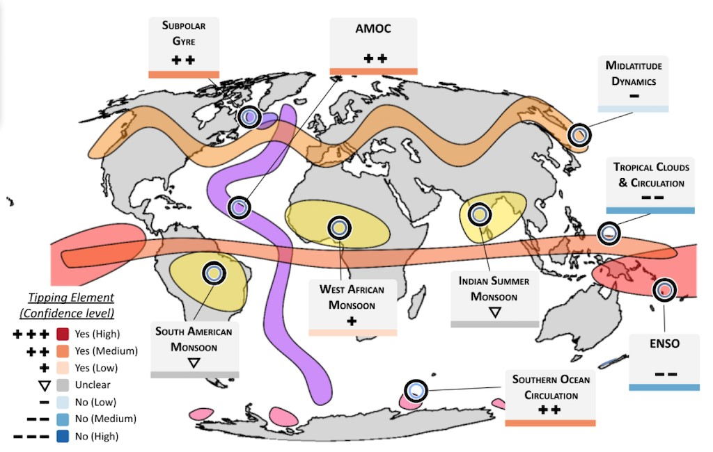
Figure II.A.7: Various ocean tipping points that may be occurring now or in the near future. Three types of transitions are included: ice-cover transitions (blue); coral reef transitions (red-orange); and kelp forest transitions (green). The transitions are also graded by climate change hazards, social vulnerabilities, and economic vulnerabilities.
There are possibilities for some mitigating circumstances that might decrease the impacts of global warming and other stresses on warm-water coral reef systems. First, it is possible that reef systems are more resilient to climate stresses than has been assumed. This is unlikely, as global reef systems have been studied widely in recent decades, and there is ample evidence of recent temporary and permanent damage to reef systems. Another possibility is that coral reefs may be able to migrate poleward, to locations where ocean temperatures are not as warm. This is limited by the fact that many elements of coral reefs have great difficulty in migrating. There is also the potential that damage to coral reef systems will exceed estimates from models. This could occur if there are correlations between different reef stressors that combine to increase the damage suffered by coral reefs. In any case, coral reef systems around the globe are experiencing serious losses due to global climate change and remain in serious jeopardy as global warming continues.
II.B: Ice Sheet Tipping Points
The majority of the Earth’s fresh water is held in what is termed the cryosphere. This is a term that refers to ice in glaciers, sea ice, and in major ice sheets such as the Greenland ice sheet and the Antarctic ice sheet. In addition, the cryosphere includes land regions where water is stored in permanent frost beds or permafrost below the Earth’s surface. These areas are found in the Arctic and Antarctic regions. Because global warming is occurring much more rapidly in the polar regions, such regions are most likely to be in danger of passing tipping points that lead to irreversible change. In this post we will discuss the condition of permafrost in section II.D.
Figure II.B.1 shows a number of ecosystems in the cryosphere. Each system is denoted by a color-coded danger level for approaching a tipping point, plus the confidence level (low, medium or high, indicated by number of + signs) that the system might be in danger. A similar rating scale is used for those systems that do not seem to be vulnerable to reaching a tipping point (denoted by – signs), plus the confidence level for that system. In this subsection, we will consider two of the areas with a high confidence level for reaching a tipping point: the Greenland ice sheet and the West Antarctic ice sheet. We will discuss these two systems separately, as the forces that are driving the systems toward tipping points are rather different for the two systems.
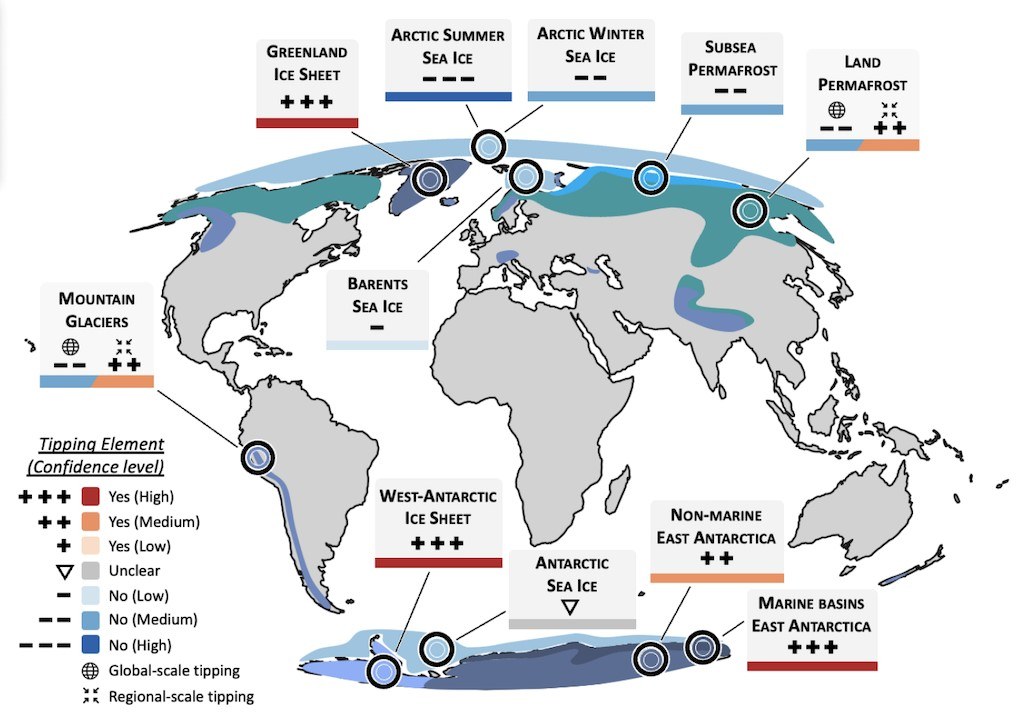
Figure II.B.1: A map of cryosphere systems around the globe. Those systems that are in danger of reaching a tipping point are denoted by “+” signs while those that are not currently in danger are denoted by “-“ signs. For each system the level of confidence is shown by the number of signs. For systems in danger of reaching a tipping point, those with high confidence are rated “+++,” while those with medium or low confidence are rated “++” and “+”, respectively. For mountain glaciers and land permafrost, the tipping probabilities are denoted separately for global vs. regional systems.
Figure II.B.2 shows topographic maps of the bedrock systems for the Greenland ice sheet (left) and the Antarctic ice sheet (right). On each map are drawn white lines. On the cross sections below are shown the bedrock and ice sheet heights along the white line. Line A is drawn across the southern area of the Greenland ice sheet (GrIS); line B is drawn across the West Antarctic ice sheet (WAIS) while line C is drawn across the East Antarctic ice sheet (EAIS). Marine ice sheet sectors, where the ice sheet rests on a bed submerged below sea level, are denoted by blue-green shading on the map.
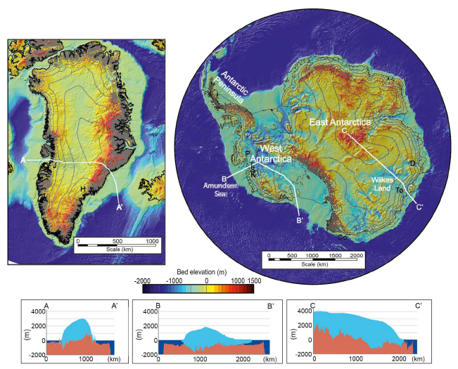
Figure II.B.2: Topography of the Greenland and Antarctic ice sheets. The upper graphs show the bedrock topography for the Greenland Ice Sheet (left) and the Antarctic Ice Sheet (right). Lines are drawn across the ice sheets. The lower graphs show the levels (in meters) of rock (brown) and ice (light blue) across the GrIS (A), the WAIS (B) and the EAIS (C). Marine ice sheet sectors, where the ice sheet rests on a bed submerged below sea level, are shown in dark blue.
The ice sheets are currently losing mass, and the rate at which mass is being lost is accelerating over time. For example, between 1992 and 1999 the average rate of loss from the Greenland ice sheet was 39 gigatonnes per year (where 1 gigatonne or Gt equals one billion metric tonnes and 1 tonne is the weight of 1000 kilograms or 1.1 English tons). During the period 2000 – 2009, the average loss was 175 Gt/yr and from 2010 – 2019, the average loss was 243 Gt/yr. The largest loss from ice sheets around the globe is currently occurring for the GrIS; between 1992 and 2020 the total mass loss was 4890 ± 850 Gt. This amount of melt contributed 13.5 mm to global sea rise. The mass loss from the Greenland and Antarctic ice sheets is approximately equal to the combined mass losses from all glaciers outside of Greenland and Antarctica. The dynamics of ice sheet systems represent the interplay of very complex driving forces. Some of these effects lead to an accelerating rate of ice mass loss, where others constitute damping forces that tend to stabilize the system.
Figure II.B.3 shows mass changes for the Greenland and Antarctic ice sheets between 2003 and 2019. Areas where mass is being lost are shown in shades of red, while areas experiencing gain in mass are shown in blue. The scale of changes is given in meters of ice equivalent per year.
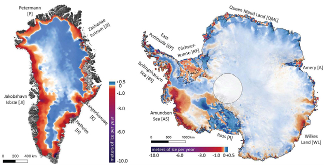
Figure II.B.3: Observed mass changes of Greenland (left) and Antarctic (right) ice sheets during the period 2003 – 2019. Red denotes areas where mass is being lost, while blue denotes areas experiencing a gain in mass. The scale of changes is in meters of ice equivalent per year.
The Greenland Ice Sheet [GrIS]:
The Greenland ice sheet is a land-based continental ice sheet with an area of 1.71 million square kilometers. At the edges of the ice sheet are outlet glaciers that release mass into the sea. The two dominant mechanisms for mass loss are increased surface melting and breaking, or calving, of glaciers at their edges. When temperatures warm the humidity increases; this causes increased precipitation in the form of snow. So central areas of the Greenland ice sheet might actually increase in mass during a warming period.
There are two loops that lead to positive feedback and an increased rate of melting of the Greenland ice sheet. The first is called the melt-elevation feedback. In this case, surface melting of the ice sheet can cause the ice sheet surface to sink to lower elevations, where the air mass is warmer. This in turn leads to increased melting. A second loop is called melt-albedo feedback. In this case, warming causes snowpack to melt to bare ice. The albedo of ice (the level of reflection for incident radiation) is smaller than for the snowpack, so the ice absorbs more of the solar radiation. This produces increased melting and a further reduction in albedo. There is a potential weak negative feedback mechanism called isostatic rebound that can operate over very long time periods. When the mass of the ice sheet decreases, this decreases the downward gravitational pressure on the underlying bedrock. The bedrock might then gradually increase in height. This exposes the ice sheet surface to cooler air temperatures and may increase the mass in the ice sheet. Models of ice sheet dynamics predict that the melt-elevation feedback loop will dominate and can produce a tipping point. Once this point is reached, it is difficult or impossible for the system to return to its previous stable state, and the melting may continue to accelerate even if global temperatures were to stabilize.
A major issue is to determine at what global temperature changes do the positive feedback drivers, particularly the melt-elevation feedback, overcome the effect of increasing snow in the center of the ice sheet and the isostatic rebound. Models of the GrIS system (here and here) suggest that global warming above preindustrial levels between 0.8o C and 3o C provide a critical threshold beyond which the ice sheet will continue to completely melt. We also have paleo record data indicating that the GrIS partially retracted during the Marine Isotope Stage 5 (MIS-5) interglacial era, that occurred roughly 120,000 years ago and was the last interglacial period before the present. It appears that the GrIS probably collapsed during the MIS-11 interglacial period that occurred about 400,000 years ago and is the warmest era in the past 500,000 years. Other models suggest that the ice sheet may re-stabilize if the global warming is less than 2o C, but for temperatures above that level the ice sheet will pass a tipping point and proceed to lose a majority of the ice.
We emphasize that the ice sheets constitute extremely complex dynamical systems, and therefore that model simulations may turn out to be incorrect. However, predicted changes in ice sheets are based on current measured losses, and should be taken seriously. In addition, it is possible that the model simulations could be underestimating the tipping dynamics. If the ice sheets pass a tipping point, then the sheets may proceed irreversibly to lose a large fraction of their mass. If either the Greenland or West Antarctic ice sheet completely melts, this would occur over a time period of a few hundred to a few thousand years. However, the results would be dire. Collapse of the Greenland ice sheet would raise global sea levels up to 7 meters, while melting of the West Antarctic ice sheet would result in global sea rise of up to 3 meters.
These levels of sea rise are so great that they would trigger other effects worldwide. For some countries, coastal areas would be completely submerged. Many Pacific Island countries would also become uninhabitable. The melting would result in the injection of a great deal of freshwater into the oceans. This would dramatically change the salinity of seawater and would disrupt the major thermohaline ocean currents, which are treated in subsection II.C. Our current state of knowledge suggests that the Greenland ice sheet is a dynamical system subject to tipping points, and that the tipping points could be reached within the next few decades or centuries, depending on the level of global warming.
The West Antarctic Ice Sheet [WAIS]:
The West Antarctic ice sheet is also losing mass at a rapid rate. Between 1992 and 1999 the average rate of loss from the West Antarctic ice sheet was 49 Gt/yr. During the period 2000 – 2009, the average loss was 70 Gt/yr and from 2010 – 2019, the average loss was 148 Gt/yr. Between 1992 and 2020 the total mass loss from the WAIS was 2670 ± 840 Gt. This amount contributed 7.4 mm to the global sea rise. Under all considered climate scenarios, both the Greenland ice sheet (with confidence level “virtually certain”) and the West Antarctic ice sheet (with confidence level “likely”) will continue to lose mass through the remainder of this century.
There are several differences in dynamics between the WAIS and the GrIS ice sheets. First, Antarctic temperatures are lower than those in Greenland; and second, the Antarctic surface is brighter than in Greenland. As a result, there is less surface melting on the Antarctic peninsula. A main cause of ice melting in the West Antarctic occurs in marine basins; these are regions where the bedrock is below sea level and is surrounded by floating ice shelves. Ocean currents flow underneath the ice shelves, and warming ocean temperatures melt the ice shelves from below. Melting of the ice shelves does not increase sea levels; since the floating ice displaces its own weight in water, when it melts the sea level does not rise. However, as the ice shelves melt, forces on the ice sheet cause grounded ice to move towards the sea. Melting of that ice does cause sea level rise. Figure II.B.4 shows two different mechanisms that contribute to increased ice melting and subsequent sea level rise. The first is called marine ice sheet instability, or MISI, shown in part A of Fig. II.B.4. In this case, “the grounding – the separation line between the grounded ice sheet and floating ice shelves – sits on retrograde bedrock slopes. If the grounding line retreats into regions of greater ice thickness, for instance due to enhanced sub-shelf melting, this increases the flux across the grounding line, leading to further retreat.”
A second type of ice sheet instability, shown in part B of Fig. II.B.4, is called marine ice-cliff instability or MICI. The hypothesis is that an ice sheet could suffer a fracture that would compel a large cliff to suddenly break off and deposit a large ice mass into the sea. We have recently observed fracturing ice sheets in West Antarctica. A group from the University of Washington observed that a 6.5-mile crack formed in about 5.5 minutes on the Pine Island Glacier, a component of the WAIS. The crack expanded at a rate of about 80 miles per hour, making it the fastest rift-opening event ever observed. The U of Washington group obtained their results by combining seismic data with results from satellite radar measurements. On other areas in Antarctica rift formation proceeds at a much slower rate than that seen on Pine Island Glacier.
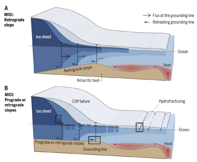
Figure II.B.4: Schematic diagrams of two processes that could contribute to Antarctic ice sheets reaching a tipping point. A) Marine ice-sheet instability or MISI. With increased sea water temperatures and rapid melt of floating ice sheets, the “grounding line” separation between the ice sheet and floating shelves can retreat. When this happens, ice sheets on bedrock can melt faster and cause sea level rise. B) Marine ice-cliff instability or MICI. Sea cliffs at the border of the ice sheet and floating ice shelves could detach and fall into the ocean, causing sea level rise and more rapid melting of the ice sheet.
It is hypothesized that the collapse of the WAIS in earlier epochs was triggered by MISI. There is also paleoclimate evidence from the Pliocene Era suggesting that the WAIS may have collapsed, leading to a 20 m increase in global sea levels. If the West Antarctic ice sheet collapses, this would lead to a rise in global sea levels of up to 3 m, over a time interval of centuries to millennia. The MICI hypothesis has not been studied as much as MISI phenomena; thus, the MICI model simulations are currently listed as being of “low confidence.”
There is historical evidence suggesting that prior collapses of the Greenland or Antarctic ice sheets produced major effects. The sea level rise that would result from melting the Greenland or Antarctic ice sheets is exceptionally high. For example, melting of the entire (West plus East) Antarctic ice sheets could raise global sea levels by as much as 58 m. In conclusion, ice sheets across the globe are rapidly melting. Glacial ice sheets are responsible for much of the water carried by the world’s largest rivers. The large-scale retreat of glaciers could be disastrous for farming communities that rely on the glaciers for irrigation, or for drinking water. In addition, large-scale melting of the ice sheets has major effects on a number of areas, affecting “sea level, ecosystems, coastal infrastructure, human livelihoods and regional climate patterns.” The release of large amounts of freshwater into the sea from melting of ice sheets can produce major disruption of worldwide ocean currents, as was discussed in our recent blog post on this issue and is described further in the following subsection. Although the complete melting of the Greenland or Antarctic ice sheets could take place over millennia, the effects on global ecosystems would be so dire that efforts to understand the dynamical forces, and to mitigate the effects of ice sheet tipping points, should be among the highest priorities for climate scientists.
II.C. North Atlantic Ocean Currents
Two potential tipping points with strong influence over the Northern Hemisphere climate are associated with coupled ocean currents in the North Atlantic. The Atlantic Meridional Overturning Circulation (AMOC) is a part of the Global Conveyor Belt of thermohaline currents we described in some detail in our previous post on Ocean Currents. The Global Conveyor Belt illustrated in Fig. II.C.1 is driven by density changes in ocean water around the globe. The water density increases as its temperature (thermo) drops and as its salinity (haline) increases. In the AMOC portion of this belt, cold salty water in the North Atlantic, around Greenland and Iceland, sinks deep below the ocean surface, and warm salty water, ultimately from the Southern Ocean, flows in along the surface to replace the sinking cold water. The new warmer water is now warmer than its surroundings, so it transfers heat to the atmosphere, cools, and then sinks itself. The heat transferred to the atmosphere helps to keep Northwestern Europe temperate. Meanwhile, the deep, cold water circulates back to the Southern Ocean, where it mixes with the warmer waters there and rises, to complete the circuit.

Figure II.C.1. The Global Conveyor Belt of thermohaline ocean currents, seen in a polar view with Antarctica near the center. Brown currents represent warm water flows along the surface, while blue currents represent cold water flow deep below the surface. The arrows indicate the directions of flow.
In the North Atlantic, the warm water flow associated with the AMOC bifurcates, as indicated in Fig. II.C.2, leading to two distinct areas where the salty water cools and sinks deep (as much as 3000 meters) beneath the surface. The approximate locations of the deepest convection sites are indicated by yellow dots in the figure, one in the Norwegian-Greenland Sea east of Greenland, and the other in the Labrador Sea south of Greenland. The surface water flow leading toward the latter deep convection site is driven by prevailing winds surrounding a low-pressure region south of Greenland. That current forms a part of the North Atlantic Subpolar Gyre, labeled SPG in Fig. II.C.2 – one of a number of surface ocean current loops around the globe. The Coriolis effect resulting from the Earth’s rotation about its axis converts air currents moving in toward a low-pressure region into counter-clockwise circulation in the Northern Hemisphere. The water flow in the SPG, therefore, circulates in a counterclockwise sense, similar to hurricanes and cyclones in the Northern Hemisphere. In our post on Ocean Currents, we dealt with the five major subtropical gyres in Earth’s oceans. The North Atlantic Subtropical Gyre is labeled by STG in Fig. II.C.2. In contrast to the SPG, the STG involves water circulation in a clockwise sense because it is driven by winds surrounding a high-pressure region in the middle of the Atlantic Ocean near 30° northern latitude.
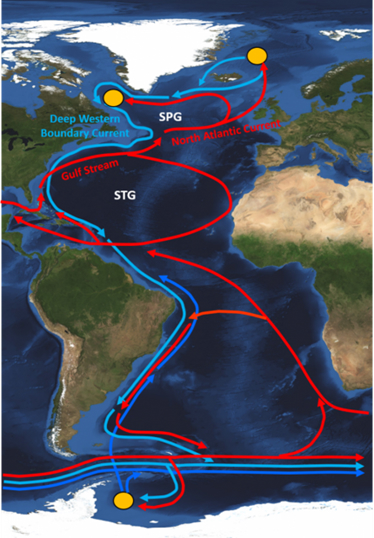
Figure II.C.2. A simplified illustration of the Atlantic Meridional Overturning Circulation and the North Atlantic Subpolar Gyre. The red arrows represent flows of warm, salty water near the surface. The blue arrows represent flows of cold, salty water deep below the surface. The yellow dots represent deep water formation areas in the Labrador Sea, the Norwegian-Greenland Sea, and the Antarctic Weddell Sea. The North Atlantic Subpolar and Subtropical Gyres are denoted by the labels SPG and STG, respectively. The cooler, upwelled surface current along the Labrador coast that completes the SPG loop is not shown. Image credit: L. Sanguineti, University of Bremen.
The Global Tipping Points Report assesses “medium confidence” in climate tipping dynamics for both the AMOC and the SPG. As in the other cases we treat in this post, tipping dynamics require positive feedback mechanisms that can amplify changes induced by global warming and eventually make them self-sustaining. The most prominent driver of AMOC and SPG weakening caused by ongoing climate change is a massive influx of fresh water into the North Atlantic, predominantly from runoff from the melting Greenland ice sheet, with additional input from melting Arctic sea ice and Arctic river discharge. We have seen in the preceding subsection that the Greenland ice sheet has its own tipping point, possibly to be reached in the coming decades, leading to a complete meltdown of the ice sheet over centuries or even millennia. The addition of fresh water reduces the salinity of the ocean surface currents in the North Atlantic and thereby disrupts the sinking of cold, salty water that is central to both AMOC and SPG. The major positive feedback mechanism that can lead to tipping in both AMOC and SPG involves salt flow from the South. As AMOC and SPG weaken, there is less influx of salty water, thereby reducing the density of the North Atlantic surface currents and further suppressing formation of the deep, cold, salty currents that drive the AMOC and SPG. In addition, reduced density of the surface water tends to weaken the convective mixing at the Labrador Sea deep water formation site, and this provides positive feedback to further weaken the SPG on a path toward its eventual collapse.
In NASA’s annual global maps of mean temperature anomalies (the one for 2022 is shown in Fig. II.C.3), there is a persistent recent cool spot in the North Atlantic just south of Greenland. The existence of this so-called “warming hole” has been attributed to weakening of the SPG and/or AMOC. In addition, there are possible indications of AMOC weakening by about 15% over the past 50 years from proxy measurements – particularly, sea surface temperatures and coastal sea levels – believed to be correlated with the AMOC. However, the Global Tipping Points Report states that “the proxy data used in these studies have large uncertainties, and some other reconstructions show little evidence of decline…The IPCC’s most recent assessment is that the AMOC has weakened relative to 1850-1900, but with low confidence due to disagreements among reconstructions…and models.” It is also noted that the large global Earth climate models may well overestimate the stability of the AMOC. Direct measurements of AMOC flow strength have been made only since 2004 and it is still too early, given the possibility for short-term variability, to glean definitive evidence regarding long-term trends.
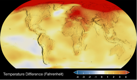
Figure II.C.3. NASA global map of mean temperatures in 2022 relative to the 1951-1980 average. Note the “hole” in the strong warming pattern at high northern latitudes just south of Greenland. The persistence of this hole has been suggested as evidence for the weakening of the North Atlantic Subpolar Gyre.
These uncertainties leave the future of the AMOC in doubt. Most models agree that the circulation will weaken substantially during the current century as the melting of Greenland ice accelerates. But the IPCC’s 6th Assessment Report assigns only “medium confidence” that an AMOC complete collapse will not happen before 2100, while judging the probability of such a collapse before 2300 to be about 50%. A recent simulation by Van Westen, et al., perturbed a detailed global climate model by introducing an adjustable input of fresh water in the North Atlantic. As shown in Fig. II.C.4, the AMOC circulation strength within their model slowly decreases as more fresh water is accumulated over the years, until a clear tipping point is reached when the cumulative fresh water input flow is just above half a million cubic meters per second. It is unclear if and when this flow rate would be reached by Greenland ice sheet melt. On the other hand, the tendency of the global climate models to overestimate AMOC stability may also have led to an overestimate in the Van Westen simulation of the fresh water input rate needed to reach the tipping point.
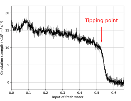
Figure II.C.4. Results of climate model simulations from van Westen, et al. that show how quickly the AMOC collapses once it reaches a tipping point with a threshold of cold fresh water flow entering the North Atlantic Ocean. Both vertical and horizontal axes are measurements of flow rates in millions of cubic meters of water per second.
There is proxy evidence that the AMOC did weaken very substantially, or possibly completely collapse, during paleoclimate episodes over the past 70,000 years. The proxy used involves measurements of long-lived isotopes from uranium decay in samples of ocean sediment that can be radioactively dated. Thorium-230 (230Th, half-life = 75,000 years) is produced in the decay of uranium-238 while protactinium-231 (231Pa, half-life = 33,000 years) is produced in the decay of uranium-235. The parent uranium is known to be well mixed throughout the ocean, and the decay production ratio is 231Pa/230Th = 0.093. Both daughter isotopes get rapidly adsorbed onto marine particles, which then get deposited on the sea floor as sediment. But, as indicated in Fig. II.C.5, the Pa-loaded sediment particles are transported southward more efficiently than the Th-loaded sediment by the deep-water flow of the AMOC. Thus, when the AMOC is strong the Pa/Th ratio in deep western North Atlantic sediment samples is reduced from the production ratio to about 0.05-0.06. When the AMOC is weak, neither the Th- nor Pa-loaded sediment is transported, so the ratio remains closer to 0.09.
Figure II.C.5. Illustration of the production rates (boxes) and water-transport rates (arrows) measured by Deng, et al., for 230Th (blue) and 231Pa (yellow) at three latitudes in the Atlantic Ocean, under current conditions when the AMOC is relatively strong. Note that only 5% of the Th, but 32% of the Pa, produced in the North Atlantic is transported to the south by the AMOC deep water component in the modern ocean.
Measurements in Fig. II.C.6 of the Pa/Th ratio (corrected for the difference in lifetime between the two isotopes) in deep sediment samples extracted from the Bermuda Rise around latitude 34° in the western North Atlantic reveal a number of AMOC weakening or collapse episodes from the past 70,000 years. The most recent narrow downward spike in the figure represents a period during the deglaciation from the last Earth Ice Age, from 12,900 to 11,600 years ago, known as the Younger Dryas. It is known to coincide with a massive influx of fresh water into the North Atlantic from the breakup and melting of the Laurentide ice sheet that covered the northern portion of North America at the Last Glacial Maximum some 21,000 years ago. It is also known from ice core samples analyzed in Greenland that the central Greenland temperature dropped rather suddenly by about 10°C during the Younger Dryas (Fig. II.C.7). Thus, we have paleoclimate evidence that the AMOC has been drastically weakened in the past by massive influx of fresh water and that weakening has caused severe changes in Northern Hemisphere climate.
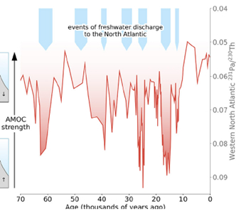
Figure II.C.6. Measurements of the 231Pa/230Th ratio in deep sea sediment samples from the Bermuda Rise region in the western North Atlantic, as a function of the inferred age of the sample. In the downward dips the ratio approaches the known production ratio for the two isotopes, indicating weak or missing AMOC transport of Pa-loaded particles. The most rightward downward spike corresponds to the Younger Dryas period and the melting of the Laurentide ice sheet.
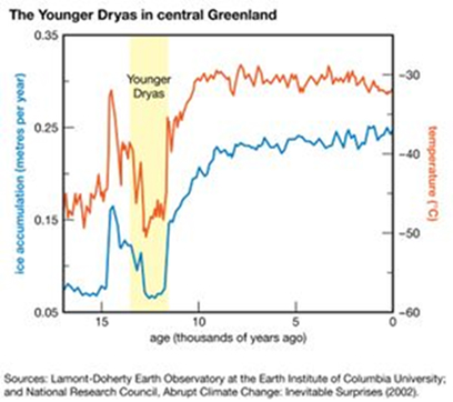
Figure II.C.7. The impact of the Younger Dryas (YD) event on ice accumulation rates (blue curve and left-hand axis) and temperatures (red curve and right-hand axis) deduced from central Greenland ice cores. Models suggest that the event was probably triggered by rapid melting of ice sheets and glaciers in the Northern Hemisphere, greatly weakening the Atlantic Meridional Overturning Circulation. The Greenland evidence shows that both temperature and snow accumulation dropped rapidly in the North Atlantic, but then recovered quickly about 11,600 years ago.
Based on currently available information and barring unforeseen rapid changes, then, the best guesses are that an AMOC tipping point and subsequent collapse are more than a century away, although there have been a few recent warnings of more imminent collapse. If it comes, however, the impacts will be drastic. There will be general cooling of the Northern Hemisphere, by up to 10°C below preindustrial levels in northwestern Europe or even 20°C in the northern reaches of Scandinavia, as per the Van Westen simulation. Southern Hemisphere temperatures would likely warm by a few degrees as less of the Southern Ocean’s heat is transported northward. An AMOC collapse would also lead to dramatic changes in storm and precipitation patterns in all tropical regions, and especially drought in the Amazon rain forest that provides an important portion of the Earth’s carbon sink. It would also lead to changes in North Atlantic sea level and reduction in its oxygen content, with serious implications for marine ecosystems. The Global Tipping Points report summarizes potential impacts this way: “An AMOC collapse would disrupt regional climates worldwide, substantially reducing vegetation and crop productivity across large areas of the world, with profound implications for food security.”
Because it takes a millennium for a water molecule to complete an AMOC circuit, the AMOC is rather resistant to rapid change. In contrast, reaching a tipping point for the SPG is expected to happen on a considerably shorter time scale, decades rather than centuries. SPG tipping is assumed to occur as a result of a collapse of the deep-water convection in the Labrador Sea south of Greenland, a collapse that can be triggered by increased fresh water input from Greenland ice melt and reduced salinity influx via a weakened AMOC. Recent climate model simulations suggest a global warming threshold for SPG collapse of 1.1—3.8°C above mean preindustrial temperatures, and the IPCC assigns high confidence to tipping within this temperature range, but only medium confidence that such tipping will occur during the 21st century. If the SPG were to collapse it would produce serious effects on North Atlantic climate (a cooling of a few degrees) and marine ecosystems. It would lead to a depletion of oxygen and an increase in acidity of the North Atlantic. It could also lead to increased concentration of carbon dioxide in the atmosphere, because under normal conditions a portion of the excess CO2 emitted by fossil fuel burning is captured within the North Atlantic and transported deep under the surface at the Labrador convection site. When the convection breaks down the CO2 can be released from the ocean surface.
II.D. Permafrost
As seen in Fig. II.C.3, the ongoing global warming is most severe at high northern latitudes. That poses a significant danger to all of the frozen ground – permafrost – near the Arctic Circle. Figure II.D.1 shows the distribution of permafrost around the Arctic Circle, dominated by northern Russia, but with sizable contributions as well from northern Canada and Alaska. The permafrost lies under about 14 million square kilometers of land in the Northern Hemisphere. Much of it lies beneath a relatively thin active layer that freezes in winter and thaws in summer months. The reason that permafrost is a serious concern for climate scientists is that it stores within it huge amounts of organic carbon, which could be released to the atmosphere if the permafrost were to thaw globally. The current estimate is that “the upper three metres of permafrost soils contain about 1,035 ± 150 GtC [Gigatonnes of carbon]…or about 50% more than today’s atmosphere.”
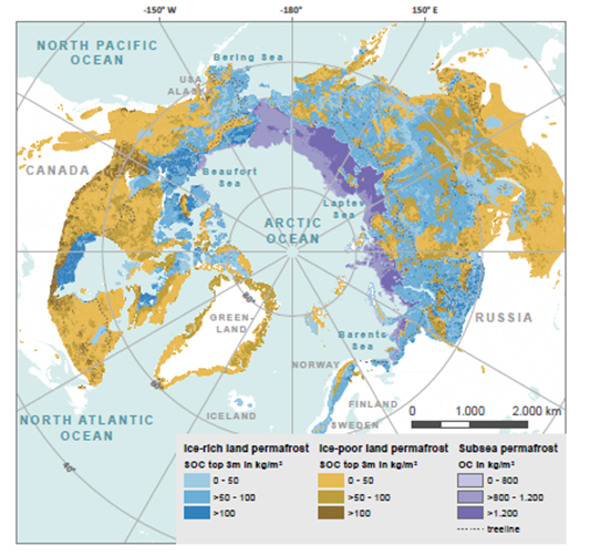
Figure II.D.1. A map of the estimated distribution of organic carbon (OC) stored within permafrost soil (SOC) or subsea permafrost in the circumpolar region. The different color shadings represent different levels of OC areal density in kilograms per square meter of permafrost area (for soil within the top 3 meters of depth). The ice-rich land permafrost is the most susceptible to rapid thawing and tipping behavior.
As illustrated in Fig. II.D.2, the positive feedback source that can potentially lead to tipping behavior involves carbon dioxide and methane released to the atmosphere from thawing permafrost, thereby enhancing the trapping of infrared radiation by greenhouse gases, increasing the warming of Earth, and amplifying the permafrost thaw. If the permafrost were to pass a tipping point it would provide a continuing source of greenhouse gas emissions even if the human burning of fossil fuels were phased out. In practice, models suggest that ice-poor land permafrost (colored in shades of brown in Fig. II.D.1) would thaw gradually, in the sense that the active upper layer of soil would grow deeper with each passing year. In such cases, the decomposition and release of stored carbon would probably take centuries, making the feedback too slow to support tipping behavior. Subsea permafrost is currently thawing at a continuous but relatively low rate and releasing carbon emissions at a rate an order of magnitude smaller than that from thawing land permafrost. So, the subsea permafrost is unlikely to have significant effect on land thawing.
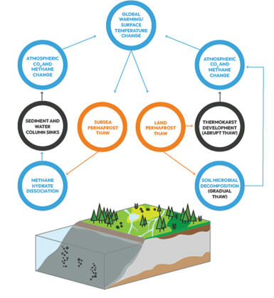
Figure II.D.2: Illustration of the positive feedback loops that could lead to tipping behavior for the thawing of the permafrost. Greenhouse gases released from thawed permafrost into the atmosphere can enhance the global warming and accelerate the thawing.
The situation is different, however, for the ice-rich land permafrost colored in shades of blue in Fig. II.D.1. As these regions, covering about 20% of the Arctic permafrost area, warm they become susceptible to rapid thawing via subsidence of the land as the ice melts and the formation of thermokarst lakes, wetlands, and gullies, as illustrated in Fig. II.D.3. The thermokarst formation is expected to release greenhouse gases much more rapidly than in ice-poor permafrost locations. Consequently, the Global Tipping Points report attaches medium confidence for tipping behavior of permafrost in local or regional areas. As of now, climate models suggest that it is unlikely that the overall greenhouse gas release from such local rapidly thawing permafrost would be sufficient to trigger a self-sustaining global thaw of the Arctic permafrost.
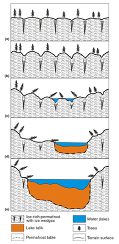
Figure II.D.3: Schematic illustration of the rapid thawing of ice-rich permafrost by subsidence of the land and formation of a thermokarst lake. Such rapid thawing can lead to local or regional tipping behavior.
Beyond enhancing greenhouse gas concentrations in the atmosphere, thawing of permafrost regions can strongly disrupt local communities. The permafrost regions are often populated, particularly by indigenous communities whose way of life is adapted to the local land, infrastructure, and food resources. Some 70% of the permafrost infrastructure is currently located in regions with high potential for thaw by 2050. Such thawing, and especially the formation of thermokarst regions, will disrupt the land topology and infrastructure, change “tundra plant and animal ecology, and the functioning of lake, river and coastal marine ecosystems…[and local] hydrological dynamics…impacting water availability and quality. These alterations, in turn, have cascading effects on the frequency and magnitude of natural disasters such as floods, landslides and coastal erosion.”
III. Summary
We are now seeing the effects of global climate change that have been predicted in the regular reports from the Intergovernmental Panel on Climate Change. We are experiencing rapidly rising temperatures, and even higher temperature changes in polar regions than at mid-latitudes. Climate-related disasters such as tornadoes, hurricanes, flooding and wildfires are increasing in severity. Our biosphere is undergoing rapid transformation as the temperature rises, sea levels rise, ice sheets shrink, and coral reefs die off. The concentration of CO2 in the atmosphere is now 50% higher than it was in pre-industrial times, and this increase is largely due to human influences. Nations are having to cope with these threats to our land, and these disasters will only increase as we continue to pour carbon dioxide and other greenhouse gases into the atmosphere.
But global climate change is also bringing the possibility for very large, and practically irreversible, changes in various aspects of the biosphere. This is the threat that various parts of our ecosystem will pass climate tipping points. The IPCC defines climate tipping points as ‘critical thresholds in a system that, when exceeded, can lead to a significant change in the state of the system, often with an understanding that the change is irreversible.’
As an example of a tipping point, consider the Greenland ice sheet. At present, as polar temperatures rapidly increase, there is increased melting of the ice sheet at the boundary with the Arctic Sea. As the surface of the ice melts, the top of the ice sheet may drop to lower elevations, where the air temperature is higher. Also, as the ice surface melts it absorbs more solar radiation, causing an increase in melting of the ice sheet. However, there are also factors that tend to slow the ice sheet melting. As the ice surface melts, this increases the humidity of the atmosphere above the ice sheet. This can lead to increased snow in the center of the ice sheet, which increases the mass of the sheet. Also, as the ice sheet melts the mass of the sheet decreases. The decreased pressure on the bedrock below may cause the ice sheet to rise to higher levels where air temperature is lower. Both of these effects can slow the melting of the ice sheet.
A 2023 500-page report from the University of Exeter has addressed the possibility that tipping points may occur in the biosphere. They have identified five different climate systems that are in greatest danger of reaching tipping points at the current levels of global climate change. Those systems are: warm-water coral reefs; the Greenland ice sheet; the West Antarctic ice sheet; the Atlantic Meridional Overturning Circulation or AMOC and the related Atlantic Subpolar Gyre; and permafrost. In this post we review all five of these systems. We discuss the rate of change in these systems and show predictions from detailed models of these systems. We estimate how close these systems may be to reaching a tipping point, and we discuss the ramifications if these systems pass a tipping point.
The results of tipping points in these systems can be extremely dangerous to the biosphere. For example, a tipping point for warm-water coral reefs could threaten the viability of these reef systems around the globe. The reefs provide homes for nearly 25% of all forms of marine life; and this marine life provides food for billions of people. The loss of a good fraction of coral reefs could imperil this source of seafood, and could also lead to catastrophic extinctions of various marine organisms. If the Greenland ice sheet were to pass a tipping point and melt entirely, this would raise sea levels by up to 7 meters. A complete melting of this ice sheet would take place over centuries or even millennia, but the results would transform our globe, inundating many Pacific islands and submerging coastal areas.
Another threat from global climate change is that a tipping point in one system might trigger tipping points in other systems, leading to chain reactions that might further threaten the ability of human and natural systems to sustain themselves. One example is the melting of the Greenland ice sheet. This has the potential to disrupt the Atlantic Meridional Overturning Current or AMOC. AMOC refers to a giant circulating system of salt water in the Atlantic, as shown schematically in Fig. II.C.2. As part of this circulating system warm water (shown in red in Fig. II.C.2) flows northeast past the eastern shores of North America; the Gulf Stream is part of this system. South of Greenland, the dense salty water cools and submerges, forming the blue currents in that figure. However, melting of the Greenland ice sheet will release large amounts of freshwater into the north Atlantic. This could weaken or stop the part of the Gulf Stream that warms western Europe altogether.
Thus, passing a tipping point in the Greenland ice sheet could trigger a second tipping point, the weakening or shutting down of the AMOC circulating system. One of the results would be dramatic drops in temperature in western Europe. Some models predict that areas of northern Finland could see temperature drops of 20o C; and agricultural production in western Europe could be devastated if the Gulf Stream were to shut down. The Exeter Global Tipping Points report stresses the possibility that a tipping point in one area of the biosphere could potentially trigger tipping points in other systems. The report calls for increased studies of the dynamics of systems in danger of passing tipping points. It calls for an international conference on tipping point dynamics, and requests that the IPCC place increased attention on tipping points in their reports.
Highlighting the danger of tipping points may cause nations to focus on efforts to slow the increase in temperature caused in large part by the increase in greenhouse gases that are emitted into the atmosphere. The March 2024 update from Berkeley Earth shows that the average temperature increase over preindustrial times is now 1.65 ± 0.11 o C. Although this is well above the 1.5 o C mark listed by the IPCC as a critical temperature increase, this may be temporary as the current El Niño system is weakening. This is likely to decrease global temperatures; however, the current temperature increases should serve as a warning that many global systems are under great stress. It is hoped that the dire results outlined in the Global Tipping Report may help stimulate nations to redouble their efforts to mitigate global climate change.
Source Material:
Global Tipping Points Report, University of Exeter 2023 https://global-tipping-points.org/
National Ocean Service, The Importance of Coral Reefs, https://oceanservice.noaa.gov/education/tutorial_corals/coral07_importance.html#:~:text=Coral%20reefs%20are%20some%20of,and%20hundreds%20of%20other%20species.
National Ocean Service, What is Coral Bleaching? https://oceanservice.noaa.gov/facts/coral_bleach.html
Climate Change, Great Barrier Reef Foundation, https://www.barrierreef.org/the-reef/threats/climate-change
European Space Agency, Understanding Climate Tipping Points, https://www.esa.int/Applications/Observing_the_Earth/Space_for_our_climate/Understanding_climate_tipping_points
Intergovernmental Panel on Climate Change (IPCC), Sixth Assessment Report (AR6), 2022 https://www.ipcc.ch/assessment-report/ar6
Abrams et al. (Accepted) ‘Committed global warming risks triggering multiple climate tipping points’, Earth’s Future. https://doi.org/10.1029/2022EF003250
Armstrong McKay, et al. (2022) ‘Exceeding 1.5°C global warming could trigger multiple climate tipping points’, Science 377(6611), p. eabn7950. https://doi.org/10.1126/science.abn7950
Beyer, H.L., et al. (2018) ‘Risk-sensitive planning for conserving coral reefs under rapid climate change’, Conservation Letters 11(6), p. e12587. https://doi.org/10.1111/conl.12587
Bland, L.M., et al. (2018) ‘Developing a standardized definition of ecosystem collapse for risk assessment’, Frontiers in Ecology and the Environment 16(1), pp. 29–36. https://doi.org/10.1002/fee.1747
Cooley, S., et al. (2023) ‘Chapter 3: Oceans and Coastal Ecosystems and their Services’, in Climate Change 2022 – Impacts, Adaptation and Vulnerability: Working Group II Contribution to the Sixth Assessment Report of the Intergovernmental Panel on Climate Change. 1st Ed’n, Cambridge, UK and New York, NY, USA: Cambridge University Press, pp. 379–550. https://doi.org/10.1017/9781009325844.005
Cooper, G.S., et al. (2020) ‘Regime shifts occur disproportionately faster in larger ecosystems’, Nature Communications 11(1), p. 1175. https://doi.org/10.1038/s41467-020-15029-x.
Cramer, K.L., et al. (2020) ‘Widespread loss of Caribbean acroporid corals was underway before coral bleaching and disease outbreaks’, Science Advances 6(17), p. eaax9395. https://doi.org/10.1126/sciadv.aax9395
Darling, E.S., et al. (2019) ‘Social–environmental drivers inform strategic management of coral reefs in the Anthropocene’, Nature Ecology & Evolution 3(9), pp. 1341–1350. https://doi.org/10.1038/s41559-019-0953-8
Dixon, A.M., et al. (2022) ‘Future loss of local-scale thermal refugia in coral reef ecosystems’, PLOS Climate 1(2), p. e0000004. https://doi.org/10.1371/journal.pclm.0000004
Frieler, K., et al. (2013) ‘Limiting global warming to 2 °C is unlikely to save most coral reefs’, Nature Climate Change 3(2), pp. 165–170. https://doi.org/10.1038/nclimate1674
Hock, K., et al. (2017) ‘Connectivity and systemic resilience of the Great Barrier Reef’, PLOS Biology 15(11), p. e2003355. https://doi.org/10.1371/journal.pbio.2003355
Hoegh-Guldberg, O., et al. (2018) ‘Impacts of 1.5oC Global Warming on Natural and Human Systems’, in Global Warming of 1.5°C. An IPCC Special Report on the impacts of global warming of 1.5°C above pre-industrial levels and related global greenhouse gas emission pathways, in the context of strengthening the global response to the threat of climate change, sustainable development, and efforts to eradicate poverty. Cambridge, UK and New York, NY, USA: Cambridge University Press, pp. 175–312. https://www.ipcc.ch/sr15/chapter/chapter-3/ (Accessed: 16 October 2023)
Houk, P., et al. (2020) ‘Predicting coral-reef futures from El Niño and Pacific Decadal Oscillation events’, Scientific Reports 10(1), p. 7735. https://doi.org/10.1038/s41598-020-64411-8
Hughes, T.P., et al. (2017) ‘Global warming and recurrent mass bleaching of corals’, Nature 543(7645), pp. 373–377. https://doi.org/10.1038/nature21707
Hughes, T.P., et al. (2018) ‘Global warming transforms coral reef assemblages’, Nature 556(7702), pp. 492–496. https://doi.org/10.1038/s41586-018-0041-2
Intergovernmental Panel on Climate Change (IPCC) (2019) Climate Change and Land: IPCC Special Report on Climate Change, Desertification, Land Degradation, Sustainable Land Management, Food Security, and Greenhouse Gas Fluxes in Terrestrial Ecosystems, Cambridge University Press https://www.ipcc.ch/srccl/cite-report/
Le Nohaïc, M., et al. (2017) ‘Marine heatwave causes unprecedented regional mass bleaching of thermally resistant corals in northwestern Australia’, Scientific Reports 7(1), p. 14999. https://doi.org/10.1038/s41598-017-14794-y
McWhorter, J.K., et al. (2022) ‘The importance of 1.5°C warming for the Great Barrier Reef’, Global Change Biology 28(4), pp. 1332–1341. https://doi.org/10.1111/gcb.15994
Muñiz-Castillo, A.I., et al. (2019) ‘Three decades of heat stress exposure in Caribbean coral reefs: a new regional delineation to enhance conservation’, Scientific Reports 9(1), p. 11013. https://doi.org/10.1038/s41598-019-47307-0
Obura, D., et al. (2022) ‘Vulnerability to collapse of coral reef ecosystems in the Western Indian Ocean’, Nature Sustainability 5(2), pp. 104–113. https://doi.org/10.1038/s41893-021-00817-0
Perry, C.T., et al. (2013) ‘Caribbean-wide decline in carbonate production threatens coral reef growth’, Nature Communications 4(1), p. 1402. https://doi.org/10.1038/ncomms2409
Setter, R.O., et al. (2022) ‘Co-occurring anthropogenic stressors reduce the timeframe of environmental viability for the world’s coral reefs’, PLOS Biology 20(10), p. e3001821. https://doi.org/10.1371/journal.pbio.3001821
Sheppard, C., et al. (2020) ‘Coral mass mortalities in the Chagos Archipelago over 40 years: Regional species and assemblage extinctions and indications of positive feedbacks’, Marine Pollution Bulletin 154, p. 111075. https://doi.org/10.1016/j.marpolbul.2020.111075
Souter, D., et al. (2021) Status of Coral Reefs of the World 2020. Global Coral Reef Monitoring Network (GCRMN) and International Coral Reef Initiative (ICRI). https://doi.org/10.59387/WOTJ9184
Vercelloni, J., et al. (2020) ‘Thresholds of Coral Cover That Support Coral Reef Biodiversity’, in K.L. Mengersen, P. Pudlo, and C.P. Robert (eds) Case Studies in Applied Bayesian Data Science: CIRM Jean-Morlet Chair, Fall 2018. Cham: Springer International Publishing (Lecture Notes in Mathematics), pp. 385–398. https://doi.org/10.1007/978-3-030-42553-1_16
Veron, J.E.N. et al. (2009) ‘The coral reef crisis: The critical importance of<350ppm CO2’, Marine Pollution Bulletin 58(10), pp. 1428–1436. https://doi.org/10.1016/j.marpolbul.2009.09.009
Wilkinson, C.R. (1999) ‘Global and local threats to coral reef functioning and existence: review and predictions’, Marine and Freshwater Research 50(8), pp. 867–878. https://doi.org/10.1071/mf99121
Plaisance, L. et al., (2011) ‘The Diversity of Coral Reefs: What Are We Missing?’, PLOS ONE 6(10), p. e25026. https://doi.org/10.1371/journal.pone.0025026
Wikipedia, El Niño – Southern Oscillation https://en.wikipedia.org/wiki/El_Ni%C3%B1o%E2%80%93Southern_Oscillation
Catrin Einhorn, The Widest-Ever Global Coral Crisis Will Hit Within Weeks, Scientists Say, New York Times, April 15, 2024 https://www.nytimes.com/2024/04/15/climate/coral-reefs-bleaching.html
B. Fox-Kemper et al. (2021) ‘Chapter 9: Ocean, Cryosphere and Sea Level Change’, in V. Masson-Delmotte, et al., Climate Change 2021: The Physical Science Basis. Contribution of Working Group I to the Sixth Assessment Report of the Intergovernmental Panel on Climate Change. Cambridge University Press https://www.ipcc.ch/report/ar6/wg1/chapter/chapter-9/
J. Oerlemans (1981) ‘Some basic experiments with a vertically-integrated ice sheet model’, Tellus 33(1), pp. 1–11. https://doi.org/10.3402/tellusa.v33i1.10690
J.E. Box et al. (2012) ‘Greenland ice sheet albedo feedback: thermodynamics and atmospheric drivers’, The Cryosphere 6(4), pp. 821–839. https://doi.org/10.5194/tc-6-821-2012
Levermann and R. Winkelman (2016) ‘A simple equation for the melt elevation feedback of ice sheets’, The Cryosphere 10(4), pp. 1799–1807. https://doi.org/10.5194/tc-10-1799-2016
Robinson et al. (2012) ‘Multistability and critical thresholds of the Greenland ice sheet’, Nature Climate Change 2(6), pp. 429–432. https://doi.org/10.1038/nclimate1449
D. Höning et al. (2023) ‘Multistability and Transient Response of the Greenland Ice Sheet to Anthropogenic CO2 Emissions’, Geophysical Research Letters 50(6), p. e2022GL101827. https://doi.org/10.1029/2022GL101827
A.J. Christ et al. (2021) ‘A multimillion-year-old record of Greenland vegetation and glacial history preserved in sediment beneath 1.4 km of ice at Camp Century’, Proceedings of the National Academy of Sciences 118(13), p. e2021442118. https://doi.org/10.1073/pnas.2021442118
J.M. Gregory et al. (2020) ‘Large and irreversible future decline of the Greenland ice sheet’, The Cryosphere 14(12), pp. 4299–4322. https://doi.org/10.5194/tc-14-4299-2020
J. Van Breedam et al. (2020) ‘Semi-equilibrated global sea-level change projections for the next 10,000 years’, Earth System Dynamics 11(4), pp. 953–976. https://doi.org/10.5194/esd-11-953-2020
C.L. Jakobs et al. (2020) ‘A benchmark dataset of in situ Antarctic surface melt rates and energy balance’, Journal of Glaciology 66(256), pp. 291–302. https://doi.org/10.1017/jog.2020.6
J. Garbe et al. (2020) ‘The hysteresis of the Antarctic Ice Sheet’, Nature 585(7826), pp. 538–544. https://doi.org/10.1038/s41586-020-2727-5
R.M. De Conto and D. Pollard (2016) ‘Contribution of Antarctica to past and future sea-level rise’, Nature 531(7596), pp. 591–597. https://doi.org/10.1038/nature17145
M.E. Weber et al. (2021) ‘Decadal-scale onset and termination of Antarctic ice-mass loss during the last deglaciation’, Nature Communications 12(1), p. 6683. https://doi.org/10.1038/s41467-021-27053-6
R.M. De Conto et al. (2021) ‘The Paris Climate Agreement and future sea-level rise from Antarctica’, Nature 593(7857), pp. 83–89. https://doi.org/10.1038/s41586-021-03427-0
Wikipedia, Greenland https://en.wikipedia.org/wiki/Greenland
Eric Ralls, Ice Sheet Fracture Sets a Speed Record in Antarctica, Earth.com, March 2, 2024 https://www.earth.com/news/ice-sheet-fracture-sets-a-speed-record-in-antarctica
DebunkingDenial, Ocean Currents, Weather, and Climate, https://debunkingdenial.com/ocean-currents-weather-and-climate/
Wikipedia, Ocean Conveyor Belt, https://en.m.wikipedia.org/wiki/File:Conveyor_belt.svg
The Atlantic Meridional Overturning Circulation (AMOC), https://race-synthese.de/the-atlantic-meridional-overturning-circulation
G. Sgubin, et al., Abrupt Cooling Over the North Atlantic in Modern Climate Models, Nature Communications 8, Article #14375 (2017), https://www.nature.com/articles/ncomms14375
L. Caesar, et al., Observed Fingerprint of a Weakening Atlantic Ocean Overturning Circulation, Nature 556, 191 (2018), https://www.nature.com/articles/s41586-018-0006-5
NASA Global Temperature Map, https://climate.nasa.gov/vital-signs/global-temperature/?intent=121
R. van Westen, H.A. Dijkstra, and M. Kliphuis, Atlantic Ocean is headed for a tipping point − once melting glaciers shut down the Gulf Stream, we would see extreme climate change within decades, study shows, The Conversation, Feb. 9, 2024, https://theconversation.com/atlantic-ocean-is-headed-for-a-tipping-point-once-melting-glaciers-shut-down-the-gulf-stream-we-would-see-extreme-climate-change-within-decades-study-shows-222834
R. van Westen, M. Kliphuis, and H.A. Dijkstra, Physics-Based Early Warning Signal Shows That AMOC is on Tipping Course, Science Advances 10, Issue 6, Feb. 9, 2024, https://www.science.org/doi/10.1126/sciadv.adk1189
L.F. Robinson, et al., Pa/Th as a (Paleo)Circulation Tracer: A North Atlantic Perspective, Past Global Changes Magazine 27, 56 (2019), https://pastglobalchanges.org/publications/pages-magazines/pages-magazine/12923
E. Böhm, et al., Strong and Deep Atlantic Meridional Overturning Circulation During the Last Glacial Cycle, Nature 517, 73 (2015), https://www.nature.com/articles/nature14059
F. Deng, et al., Evolution of 231Pa and 230Th in Overflow Waters of the North Atlantic, Biogeosciences 15, 7299 (2018), https://bg.copernicus.org/articles/15/7299/2018/
Brittanica, Younger Dryas, https://www.britannica.com/science/Younger-Dryas-climate-interval
Abrupt Climate Change (National Academies Press, 2002), https://nap.nationalacademies.org/catalog/10136/abrupt-climate-change-inevitable-surprises
P. Ditlevsen and S. Ditlevsen, Warning of a Forthcoming Collapse of the Atlantic Meridional Overturning Circulation, Nature Communications 14, Article #4254 (2023), https://www.nature.com/articles/s41467-023-39810-w
G. Hugelius, et al., Estimated Stocks of Circumpolar Permafrost Carbon with Quantified Uncertainty Ranges and Identified Data Gaps, Biogeosciences 11, 6573 (2014), https://bg.copernicus.org/articles/11/6573/2014/
